วิธีการวนซ้ำแบบอยู่กับที่จะแก้ระบบสมการเชิงเส้นโดยใช้ตัวดำเนินการประมาณค่าของตัวดำเนินการเดิม และจากค่าความคลาดเคลื่อนในผลลัพธ์ ( ค่าตกค้าง ) จะสร้าง "สมการแก้ไข" ซึ่งกระบวนการนี้จะถูกทำซ้ำ แม้ว่าวิธีการเหล่านี้จะง่ายต่อการคิดค้น นำไปใช้ และวิเคราะห์ แต่การลู่เข้าจะรับประกันได้เฉพาะกับเมทริกซ์บางประเภทเท่านั้น

วิธีการวนซ้ำถูกกำหนดโดย $${\displaystyle \mathbf {x} ^{k+1}:=\Psi (\mathbf {x} ^{k}),\quad k\geq 0}$$ และสำหรับระบบเชิงเส้นที่กำหนด${\displaystyle A\mathbf {x} =\mathbf {b} }$พร้อมวิธีแก้ปัญหาที่แม่นยำ${\displaystyle \mathbf {x} ^{*}}$ข้อผิดพลาดโดย $${\displaystyle \mathbf {e} ^{k}:=\mathbf {x} ^{k}-\mathbf {x} ^{*},\quad k\geq 0.}$$ วิธีการวนซ้ำเรียกว่าเชิงเส้นถ้ามีเมทริกซ์อยู่${\displaystyle C\in \mathbb {R} ^{n\times n}}$โดยที่ $${\displaystyle \mathbf {e} ^{k+1}=C\mathbf {e} ^{k}\quad \forall k\geq 0}$$ และเมทริกซ์นี้เรียกว่าเมทริกซ์การวนซ้ำวิธีการวนซ้ำโดยใช้เมทริกซ์การวนซ้ำที่กำหนดให้${\displaystyle C}$ is called convergent if the following holds $${\displaystyle \lim _{k\to \infty }C^{k}=0.}$$

An important theorem states that for a given iterative method and its iteration matrix ${\displaystyle C}$ it is convergent if and only if its spectral radius${\displaystyle \rho (C)}$ is smaller than unity, that is, $${\displaystyle \rho (C)<1.}$$

The basic iterative methods work by splitting the matrix ${\displaystyle A}$ into $${\displaystyle A=M-N}$$ and here the matrix ${\displaystyle M}$ should be easily invertible. The iterative methods are now defined as $${\displaystyle M\mathbf {x} ^{k+1}=N\mathbf {x} ^{k}+\mathbf {b} ,\quad k\geq 0,}$$ or, equivalently, $${\displaystyle \mathbf {x} ^{k+1}=\mathbf {x} ^{k}+M^{-1}\left(\mathbf {b} -A\mathbf {x} ^{k}\right),\quad k\geq 0.}$$ From this follows that the iteration matrix is given by $${\displaystyle C=I-M^{-1}A=M^{-1}N.}$$

Basic examples of stationary iterative methods use a splitting of the matrix ${\displaystyle A}$ such as $${\displaystyle A=D+L+U\,,\quad D:=\operatorname {diag} ((a_{ii})_{i})}$$ where ${\displaystyle D}$ is only the diagonal part of ${\displaystyle A}$, and ${\displaystyle L}$ is the strict lower triangular part of ${\displaystyle A}$. Respectively, ${\displaystyle U}$ is the strict upper triangular part of ${\displaystyle A}$.

• Richardson method: $${\displaystyle M:={\frac {1}{\omega }}I\quad (\omega \neq 0)}$$
• Jacobi method: $${\displaystyle M:=D}$$
• Damped Jacobi method: $${\displaystyle M:={\frac {1}{\omega }}D\quad (\omega \neq 0)}$$
• Gauss–Seidel method: $${\displaystyle M:=D+L}$$
• Successive over-relaxation method (SOR): $${\displaystyle M:={\frac {1}{\omega }}D+L\quad (\omega \neq 0)}$$
• Symmetric successive over-relaxation (SSOR): $${\displaystyle M:={\frac {1}{\omega \left(2-\omega \right)}}\left(D+\omega L\right)D^{-1}\left(D+\omega U\right)\quad (\omega \not \in \{0,2\})}$$

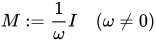
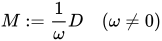
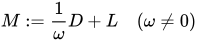
Linear stationary iterative methods are also called relaxation methods.

Since these methods form a basis, it is evident that the method converges in N iterations, where N is the system size. However, in the presence of rounding errors this statement does not hold; moreover, in practice N can be very large, and the iterative process reaches sufficient accuracy already far earlier. The analysis of these methods is hard, depending on a complicated function of the spectrum of the operator.