
ความแปรปรวนร่วม
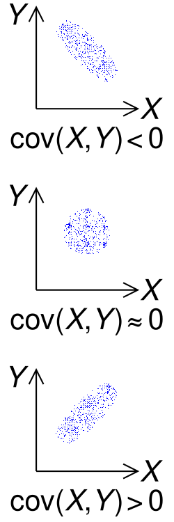
ในทฤษฎีความน่าจะเป็นและสถิติความแปรปรวน ร่วม เป็นการวัดความแปรปรวน ร่วม ของตัวแปรสุ่ม สอง ตัว[ 1 ]เครื่องหมาย ของความแปรปรวน ร่วมแสดงแนวโน้มในความสัมพันธ์เชิงเส้นระหว่างตัวแปร ความแปรปรวนร่วมเป็นบวกเมื่อตัวแปรมีแนวโน้มที่จะแสดงพฤติกรรมที่คล้ายคลึงกัน และเป็นลบเมื่อตัวแปรมีแนวโน้มที่จะแสดงพฤติกรรมตรงกันข้าม[ 2 ]ขนาดของความแปรปรวนร่วมคือค่าเฉลี่ยเรขาคณิต ของความแปรปรวนที่แบ่งปันกันสำหรับตัวแปรสุ่มสองตัว โดยขนาด ที่มากขึ้นหมายความว่าตัวแปรสองตัวนั้นขึ้นอยู่ซึ่งกันและกันอย่างแน่นแฟ้นยิ่งขึ้น
ค่าความแปรปรวนร่วมมีหน่วยวัด และขนาดของค่าความแปรปรวนร่วมจะได้รับผลกระทบจากหน่วยดังกล่าว ซึ่งหมายความว่าการเปลี่ยนหน่วย (เช่น จากเมตรเป็นมิลลิเมตร) จะทำให้ค่าความแปรปรวนร่วมเปลี่ยนแปลงไปตามสัดส่วน ทำให้ยากที่จะประเมินความแข็งแกร่งของความสัมพันธ์จากค่าความแปรปรวนร่วมเพียงอย่างเดียว ในบางสถานการณ์ เป็นที่พึงปรารถนาที่จะเปรียบเทียบความแข็งแกร่งของความสัมพันธ์ร่วมกันระหว่างตัวแปรสุ่มคู่ต่างๆ ที่ไม่จำเป็นต้องมีหน่วยเดียวกัน[ 3 ]ในสถานการณ์เหล่านั้น เราใช้สัมประสิทธิ์สหสัมพันธ์ซึ่งจะทำให้ค่าความแปรปรวนร่วมเป็นค่าระหว่าง -1 ถึง 1 โดยการหารด้วยค่าเฉลี่ยเรขาคณิตของความแปรปรวน ทั้งหมด (เช่น ผลคูณของส่วนเบี่ยงเบนมาตรฐาน ) สำหรับตัวแปรสุ่มทั้งสอง[ 4 ]
มีการแยกความแตกต่างระหว่าง (1) ความแปรปรวนร่วมของตัวแปรสุ่มสองตัว ซึ่งเป็นพารามิเตอร์ประชากร ที่สามารถมองได้ว่าเป็นคุณสมบัติของการแจกแจงความน่าจะเป็นร่วมและ (2) ความแปรปรวนร่วมของตัวอย่างซึ่งนอกจากจะทำหน้าที่เป็นตัวอธิบายของตัวอย่างแล้ว ยังทำหน้าที่เป็น ค่า ประมาณของพารามิเตอร์ประชากร อีกด้วย
คำนิยาม
สำหรับตัวแปรสุ่มค่าจริง สองตัว ที่มีการแจกแจงร่วมกันและด้วยโมเมนต์ที่สอง ที่จำกัด ความแปรปรวนร่วมจะถูกกำหนดเป็นค่าที่คาดหวัง (หรือค่าเฉลี่ย) ของผลคูณของค่าเบี่ยงเบนจากค่าที่คาดหวังของแต่ละบุคคล: [ 5 ] [ 6 ] : 119


![{\displaystyle \operatorname {cov} (X,Y)=\operatorname {E} {{\big [}(X-\operatorname {E} [X])(Y-\operatorname {E} [Y]){\big ]}}}](https://wikimedia.org/api/rest_v1/media/math/render/svg/f98a8bf924edb41a8025b5ffaa1b255b4a6f48b9)
ที่ไหนคือค่าที่คาดหวังของหรือเรียกอีกอย่างว่าค่าเฉลี่ยของค่าความแปรปรวนร่วมบางครั้งก็ถูกแสดงด้วยสัญลักษณ์อื่นเช่นกันหรือในทำนองเดียวกับความแปรปรวนโดยใช้คุณสมบัติความเป็นเส้นตรงของค่าคาดหวัง สามารถลดรูปให้เหลือเพียงค่าคาดหวังของผลคูณลบด้วยผลคูณของค่าคาดหวัง: เอกลักษณ์นี้มีประโยชน์สำหรับการพิสูจน์ทางคณิตศาสตร์ อย่างไรก็ตาม จากมุมมองของการคำนวณเชิงตัวเลข มันอาจเกิดการหักล้างกันอย่างรุนแรงได้ (ดูส่วนเกี่ยวกับการคำนวณเชิงตัวเลขด้านล่าง)
![{\displaystyle \operatorname {E} [X]}](https://wikimedia.org/api/rest_v1/media/math/render/svg/44dd294aa33c0865f58e2b1bdaf44ebe911dbf93)


![{\displaystyle {\begin{aligned}\operatorname {cov} (X,Y)&=\operatorname {E} \left[\left(X-\operatorname {E} \left[X\right]\right)\left(Y-\operatorname {E} \left[Y\right]\right)\right]\\&=\operatorname {E} \left[XY-X\operatorname {E} \left[Y\right]-\operatorname {E} \left[X\right]Y+\operatorname {E} \left[X\right]\operatorname {E} \left[Y\right]\right]\\&=\operatorname {E} \left[XY\right]-\operatorname {E} \left[X\right]\operatorname {E} \left[Y\right]-\operatorname {E} \left[X\right]\operatorname {E} \left[Y\right]+\operatorname {E} \left[X\right]\operatorname {E} \left[Y\right]\\&=\operatorname {E} \left[XY\right]-\operatorname {E} \left[X\right]\operatorname {E} \left[Y\right].\end{aligned}}}](https://wikimedia.org/api/rest_v1/media/math/render/svg/7331bb9b6e36128d1d9cb735b11b65427929105d)
หน่วยวัดของความแปรปรวนร่วมคือสิ่งเหล่านั้นของครั้งของเวลาของในทางตรงกันข้ามค่าสัมประสิทธิ์สหสัมพันธ์ซึ่งขึ้นอยู่กับค่าความแปรปรวนร่วม เป็น มาตรวัดความสัมพันธ์เชิงเส้น ที่ไม่มีมิติ (อันที่จริง ค่าสัมประสิทธิ์สหสัมพันธ์สามารถเข้าใจได้ง่ายๆ ว่าเป็นค่าความแปรปรวนร่วมที่ถูกทำให้เป็นมาตรฐานแล้ว)

ตัวแปรสุ่มเชิงซ้อน
ความแปรปรวนร่วมระหว่างตัวแปรสุ่มเชิงซ้อน สองตัวถูกกำหนดเป็น[ 6 ] : 119

![{\displaystyle \operatorname {cov} (Z,W)=\operatorname {E} \left[(Z-\operatorname {E} [Z]){\overline {(W-\operatorname {E} [W])}}\right]=\operatorname {E} \left[Z{\overline {W}}\right]-\operatorname {E} [Z]\operatorname {E} \left[{\overline {W}}\right]}](https://wikimedia.org/api/rest_v1/media/math/render/svg/cc823fe25634365b1859a3ee206ca894203a9ee2)
โปรดสังเกตการผันเชิงซ้อนของตัวประกอบที่สองในคำนิยาม
สามารถกำหนดความแปรปรวนร่วมเทียมที่เกี่ยวข้อง ได้เช่นกัน
ตัวแปรสุ่มแบบไม่ต่อเนื่อง
ถ้าคู่ตัวแปรสุ่ม (จริง)สามารถรับเอาค่านิยมเหล่านั้นได้สำหรับโดยมีความน่าจะเป็นเท่ากันดังนั้น ค่าความแปรปรวนร่วมจึงสามารถเขียนได้ในรูปของค่าเฉลี่ยได้เช่นกันและเช่น


![{\displaystyle \operatorname {E} [Y]}](https://wikimedia.org/api/rest_v1/media/math/render/svg/639e8577c6faffc0471c7e123ead30970034e6d5)

นอกจากนี้ยังสามารถแสดงได้อย่างเทียบเท่าโดยไม่ต้องอ้างอิงถึงวิธีการโดยตรง ดังนี้[ 7 ]

โดยทั่วไปแล้ว หากมีความเป็นไปได้ของการเกิดขึ้นกล่าวคือแต่มีโอกาสเกิดขึ้นไม่เท่ากันสำหรับดังนั้นค่าความแปรปรวนร่วมคือ



ในกรณีที่ตัวแปรสุ่มสองตัวแยกจากกันและมีการกระจายความน่าจะเป็นร่วมกัน ซึ่งแสดงด้วยองค์ประกอบต่างๆซึ่งสอดคล้องกับความน่าจะเป็นร่วมของค่าความแปรปรวนร่วมจะคำนวณโดยใช้ผลรวมสองชั้นเหนือดัชนีของเมทริกซ์:


![{\displaystyle \operatorname {cov} (X,Y)=\sum _{i=1}^{n}\sum _{j=1}^{n}p_{i,j}(x_{i}-E[X])(y_{j}-E[Y]).}](https://wikimedia.org/api/rest_v1/media/math/render/svg/b036eb4d41b2fb6291fda39c942f5720f4cf3329)
ตัวอย่าง
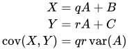
พิจารณาตัวแปรสุ่มอิสระสามตัวและค่าคงที่สองค่า. ในกรณีพิเศษและความแปรปรวนร่วมระหว่างและเป็นเพียงความแปรปรวนของและชื่อ "ความแปรปรวนร่วม" นั้นเหมาะสมอย่างยิ่ง




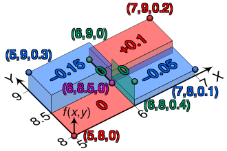
สมมติว่าและมีฟังก์ชันมวลความน่าจะเป็นร่วม ดังต่อไปนี้ [ 8 ]ซึ่งเซลล์กลางทั้งหกเซลล์ให้ความน่าจะเป็นร่วมแบบไม่ต่อเนื่องจากสถานการณ์สมมติทั้งหกประการ:


| x | ||||||
|---|---|---|---|---|---|---|
| 5 | 6 | 7 | ||||
| y | 8 | 0 | 0.4 | 0.1 | 0.5 | |
| 9 | 0.3 | 0 | 0.2 | 0.5 | ||
| 0.3 | 0.4 | 0.3 | 1 | |||


สามารถมีค่าได้สามค่า (5, 6 และ 7) ในขณะที่สามารถรับได้สอง (8 และ 9) ค่าเฉลี่ยของพวกเขาคือและ. แล้ว,


![{\displaystyle {\begin{aligned}\operatorname {cov} (X,Y)={}&\sigma _{XY}=\sum _{(x,y)\in S}f(x,y)\left(x-\mu _{X}\right)\left(y-\mu _{Y}\right)\\[4pt]={}&(0)(5-6)(8-8.5)+(0.4)(6-6)(8-8.5)+(0.1)(7-6)(8-8.5)+{}\\[4pt]&(0.3)(5-6)(9-8.5)+(0)(6-6)(9-8.5)+(0.2)(7-6)(9-8.5)\\[4pt]={}&{-0.1}\;.\end{aligned}}}](https://wikimedia.org/api/rest_v1/media/math/render/svg/8a80fa4db641ca7ddd6f7a3fee8620eed15321a7)
คุณสมบัติ
ความแปรปรวนร่วมกับตัวมันเอง
ความแปรปรวนเป็นกรณีพิเศษของความแปรปรวนร่วมซึ่งตัวแปรทั้งสองเหมือนกัน: [ 6 ] : 121

ความแปรปรวนร่วมของผลรวมเชิงเส้น
ถ้า,,, และเป็นตัวแปรสุ่มค่าจริง และถ้า เป็นค่าคงที่ที่มีค่าเป็นจำนวนจริง ข้อเท็จจริงต่อไปนี้จึงเป็นผลสืบเนื่องมาจากนิยามของความแปรปรวนร่วม:


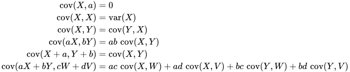
สำหรับลำดับของตัวแปรสุ่มและค่าคงที่ที่เป็นจำนวนจริงเรามี


เอกลักษณ์ความแปรปรวนร่วมของ Hoeffding
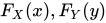
สูตรที่มีประโยชน์ในการคำนวณค่าความแปรปรวนร่วมระหว่างตัวแปรสุ่มสองตัว คือเอกลักษณ์ความแปรปรวนร่วมของ Hoeffding: [ 9 ] ที่ไหนคือฟังก์ชันการกระจายสะสมร่วมของเวกเตอร์สุ่มและคือกลุ่มชายขอบ



ความไม่สัมพันธ์กันและความเป็นอิสระ
ตัวแปรสุ่มที่มีเมทริกซ์ความแปรปรวนร่วมเป็นศูนย์เรียกว่าไม่มีความสัมพันธ์กัน[ 6 ] : 121ในทำนองเดียวกัน ส่วนประกอบของเวกเตอร์สุ่มที่มีเมทริกซ์ความแปรปรวนร่วมเป็นศูนย์ในทุกรายการนอกแนวทแยงหลักก็เรียกว่าไม่มีความสัมพันธ์กันเช่นกัน
ถ้าและหากตัวแปรสุ่มอิสระกันค่าความแปรปรวนร่วมจะเป็นศูนย์[ 6 ] : 123 [ 10 ]ซึ่งเป็นผลมาจากความเป็นอิสระ
![{\displaystyle \operatorname {E} [XY]=\operatorname {E} [X]\cdot \operatorname {E} [Y].}](https://wikimedia.org/api/rest_v1/media/math/render/svg/c0c2870ec57051083bd6262aa4069a2500dfda44)
อย่างไรก็ตาม ในทางกลับกันนั้นโดยทั่วไปแล้วไม่เป็นเช่นนั้น ตัวอย่างเช่น สมมติว่ามีการกระจายอย่างสม่ำเสมอในและปล่อยให้ชัดเจนและไม่เป็นอิสระ แต่
![{\displaystyle [-1,1]}](https://wikimedia.org/api/rest_v1/media/math/render/svg/51e3b7f14a6f70e614728c583409a0b9a8b9de01)

![{\displaystyle {\begin{aligned}\operatorname {cov} (X,Y)&=\operatorname {cov} \left(X,X^{2}\right)\\&=\operatorname {E} \left[X\cdot X^{2}\right]-\operatorname {E} [X]\cdot \operatorname {E} \left[X^{2}\right]\\&=\operatorname {E} \left[X^{3}\right]-\operatorname {E} [X]\operatorname {E} \left[X^{2}\right]\\&=0-0\cdot \operatorname {E} [X^{2}]\\&=0.\end{aligned}}}](https://wikimedia.org/api/rest_v1/media/math/render/svg/19b6f2d636d5ef9ba85b6350e49222109a28d665)
ในกรณีนี้ ความสัมพันธ์ระหว่างและความสัมพันธ์และค่าความแปรปรวนร่วมเป็นการวัดการพึ่งพาเชิงเส้นระหว่างตัวแปรสุ่มสองตัวแบบไม่เป็นเชิงเส้น ตัวอย่างนี้แสดงให้เห็นว่าหากตัวแปรสุ่มสองตัวไม่มีความสัมพันธ์กัน โดยทั่วไปแล้วไม่ได้หมายความว่าตัวแปรเหล่านั้นเป็นอิสระต่อกัน อย่างไรก็ตาม หากตัวแปรสองตัวมีการแจกแจงแบบปกติร่วมกัน (แต่ไม่ใช่หากตัวแปรแต่ละตัวมีการแจกแจงแบบปกติ เพียงอย่างเดียว ) การไม่มีความสัมพันธ์กันจะหมายถึงความเป็นอิสระ[ 11 ]
และตัวแปรที่มีค่าความแปรปรวนร่วมเป็นบวกเรียกว่ามีความสัมพันธ์เชิงบวก ซึ่งหมายความว่า ถ้าแล้วก็มีแนวโน้มว่าในทางกลับกันและค่าความแปรปรวนร่วมที่เป็นลบจะมีความสัมพันธ์กันในเชิงลบ และถ้าแล้วก็มีแนวโน้มว่า.
![{\displaystyle X>E[X]}](https://wikimedia.org/api/rest_v1/media/math/render/svg/166d8f9cb60b8835b723e34645e1f0c52a1852a5)
![{\displaystyle Y>E[Y]}](https://wikimedia.org/api/rest_v1/media/math/render/svg/02c197c6857af01266e2ed7c29485cad5a15118d)
![{\displaystyle Y<E[Y]}](https://wikimedia.org/api/rest_v1/media/math/render/svg/3eef3a2a3d98417f1d7684c3a6e530909c1c7c73)
ความสัมพันธ์กับผลิตภัณฑ์ภายใน
คุณสมบัติหลายประการของความแปรปรวนร่วมสามารถแยกออกมาได้อย่างงดงามโดยการสังเกตว่ามันมีคุณสมบัติคล้ายคลึงกับคุณสมบัติของผลคูณภายใน :
- ไบลิเนียร์ : สำหรับค่าคงที่และและตัวแปรสุ่ม
- สมมาตร:
- บวกกึ่งแน่นอน :สำหรับตัวแปรสุ่มทั้งหมด, และหมายความว่ามีค่าคงที่เกือบแน่นอน






In fact these properties imply that the covariance defines an inner product over the quotient vector space obtained by taking the subspace of random variables with finite second moment and identifying any two that differ by a constant. (This identification turns the positive semi-definiteness above into positive definiteness.) That quotient vector space is isomorphic to the subspace of random variables with finite second moment and mean zero; on that subspace, the covariance is exactly the L2 inner product of real-valued functions on the sample space.
As a result, for random variables with finite variance, the inequality is a special case of the Cauchy–Schwarz inequality.

For convenience, here is an explicit proof, which uses only the inner product properties above.
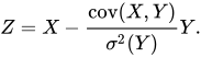
If , then it holds trivially. Otherwise, define the random variable

Then we have
![{\displaystyle {\begin{aligned}0\leq \sigma ^{2}(Z)&=\operatorname {cov} \left(X-{\frac {\operatorname {cov} (X,Y)}{\sigma ^{2}(Y)}}Y,\;X-{\frac {\operatorname {cov} (X,Y)}{\sigma ^{2}(Y)}}Y\right)\\[12pt]&=\sigma ^{2}(X)-{\frac {(\operatorname {cov} (X,Y))^{2}}{\sigma ^{2}(Y)}}\\\implies (\operatorname {cov} (X,Y))^{2}&\leq \sigma ^{2}(X)\sigma ^{2}(Y)\\\left|\operatorname {cov} (X,Y)\right|&\leq {\sqrt {\sigma ^{2}(X)\sigma ^{2}(Y)}}\end{aligned}}}](https://wikimedia.org/api/rest_v1/media/math/render/svg/ba7ff8e39a20c6976e9d6a88b8c8f95dec1385f7)
Calculating the sample covariance
The sample covariances among variables based on observations of each, drawn from an otherwise unobserved population, are given by the matrix with the entries


![{\displaystyle \textstyle {\overline {\mathbf {q} }}=\left[q_{jk}\right]}](https://wikimedia.org/api/rest_v1/media/math/render/svg/cb28ac928a2a379d039d27fb99d56dd21c1c027c)

which is an estimate of the covariance between variable and variable .


The sample mean and the sample covariance matrix are unbiased estimates of the mean and the covariance matrix of the random vector, a vector whose jth element is one of the random variables. The reason the sample covariance matrix has in the denominator rather than is essentially that the population mean is not known and is replaced by the sample mean . If the population mean is known, the analogous unbiased estimate is given by




- .

Generalizations
Auto-covariance matrix of real random vectors
For a vector of jointly distributed random variables with finite second moments, its auto-covariance matrix (also known as the variance–covariance matrix or simply the covariance matrix) (also denoted by or ) is defined as[12]:335



![{\displaystyle {\begin{aligned}\operatorname {K} _{\mathbf {XX} }=\operatorname {cov} (\mathbf {X} ,\mathbf {X} )&=\operatorname {E} \left[(\mathbf {X} -\operatorname {E} [\mathbf {X} ])(\mathbf {X} -\operatorname {E} [\mathbf {X} ])^{\mathrm {T} }\right]\\&=\operatorname {E} \left[\mathbf {XX} ^{\mathrm {T} }\right]-\operatorname {E} [\mathbf {X} ]\operatorname {E} [\mathbf {X} ]^{\mathrm {T} }.\end{aligned}}}](https://wikimedia.org/api/rest_v1/media/math/render/svg/15725714f72a46ffb0686bafdb209260b842ac39)
Let be a random vector with covariance matrix Σ, and let A be a matrix that can act on on the left. The covariance matrix of the matrix-vector product A X is:

![{\displaystyle {\begin{aligned}\operatorname {cov} (\mathbf {AX} ,\mathbf {AX} )&=\operatorname {E} \left[\mathbf {AX(A} \mathbf {X)} ^{\mathrm {T} }\right]-\operatorname {E} [\mathbf {AX} ]\operatorname {E} \left[(\mathbf {A} \mathbf {X} )^{\mathrm {T} }\right]\\&=\operatorname {E} \left[\mathbf {AXX} ^{\mathrm {T} }\mathbf {A} ^{\mathrm {T} }\right]-\operatorname {E} [\mathbf {AX} ]\operatorname {E} \left[\mathbf {X} ^{\mathrm {T} }\mathbf {A} ^{\mathrm {T} }\right]\\&=\mathbf {A} \operatorname {E} \left[\mathbf {XX} ^{\mathrm {T} }\right]\mathbf {A} ^{\mathrm {T} }-\mathbf {A} \operatorname {E} [\mathbf {X} ]\operatorname {E} \left[\mathbf {X} ^{\mathrm {T} }\right]\mathbf {A} ^{\mathrm {T} }\\&=\mathbf {A} \left(\operatorname {E} \left[\mathbf {XX} ^{\mathrm {T} }\right]-\operatorname {E} [\mathbf {X} ]\operatorname {E} \left[\mathbf {X} ^{\mathrm {T} }\right]\right)\mathbf {A} ^{\mathrm {T} }\\&=\mathbf {A} \Sigma \mathbf {A} ^{\mathrm {T} }.\end{aligned}}}](https://wikimedia.org/api/rest_v1/media/math/render/svg/c1b2123c32a8acefc209a4f69d571ee1197a8c59)
This is a direct result of the linearity of expectation and is useful when applying a linear transformation, such as a whitening transformation, to a vector.
Cross-covariance matrix of real random vectors
For real random vectors and , the cross-covariance matrix is equal to[12]:336


| Eq.2 |
![{\displaystyle {\begin{aligned}\operatorname {K} _{\mathbf {X} \mathbf {Y} }=\operatorname {cov} (\mathbf {X} ,\mathbf {Y} )&=\operatorname {E} \left[(\mathbf {X} -\operatorname {E} [\mathbf {X} ])(\mathbf {Y} -\operatorname {E} [\mathbf {Y} ])^{\mathrm {T} }\right]\\&=\operatorname {E} \left[\mathbf {X} \mathbf {Y} ^{\mathrm {T} }\right]-\operatorname {E} [\mathbf {X} ]\operatorname {E} [\คณิตศาสตร์ {Y} ]^{\คณิตศาสตร์ {T} }\end{aligned}}}](https://wikimedia.org/api/rest_v1/media/math/render/svg/99e6f5ef675f7bb826d04f206bd212d14632ab8c)
where is the transpose of the vector (or matrix) .


The -th element of this matrix is equal to the covariance between the i-th scalar component of and the j-th scalar component of . In particular, is the transpose of .


Cross-covariance sesquilinear form of random vectors in a real or complex Hilbert space
More generally let and , be Hilbert spaces over or with anti linear in the first variable, and let be resp. valued random variables. Then the covariance of and is the sesquilinear form on (anti linear in the first variable) given by




![{\displaystyle {\begin{aligned}\operatorname {K} _{X,Y}(h_{1},h_{2})=\operatorname {cov} (\mathbf {X} ,\mathbf {Y} )(h_{1},h_{2})&=\operatorname {E} \left[\langle h_{1},(\mathbf {X} -\ชื่อผู้ดำเนินการ {E} [\mathbf {X} ])\rangle _{1}\langle (\mathbf {Y} -\ชื่อผู้ดำเนินการ {E} [\mathbf {Y} ]),h_{2}\rangle _{2}\right]\\&=\ชื่อผู้ดำเนินการ {E} [\langle h_{1},\mathbf {X} \rangle _{1}\langle \mathbf {Y} ,h_{2}\rangle _{2}]-\ชื่อผู้ดำเนินการ {E} [\langle h,\mathbf {X} \rangle _{1}]\ชื่อผู้ดำเนินการ {E} [\langle \mathbf {Y} ,h_{2}\rangle _{2}]\\&=\langle h_{1},\ชื่อผู้ดำเนินการ {E} \left[(\mathbf {X} -\ชื่อผู้ดำเนินการ {E} [\mathbf {X} ])(\mathbf {Y} -\operatorname {E} [\mathbf {Y} ])^{\dagger }\right]h_{2}\rangle _{1}\\&=\langle h_{1},\left(\operatorname {E} [\mathbf {X} \mathbf {Y} ^{\dagger }]-\operatorname {E} [\mathbf {X} ]\ชื่อผู้ดำเนินการ {E} [\mathbf {Y} ]^{\dagger }\right)h_{2}\rangle _{1}\\\end{aligned}}}](https://wikimedia.org/api/rest_v1/media/math/render/svg/a5e62db23468fadd6a7f877ed44ede2bfbc07365)
Numerical computation
When , the equation is prone to catastrophic cancellation if and are not computed exactly and thus should be avoided in computer programs when the data has not been centered before.[13]Numerically stable algorithms should be preferred in this case.[14]
![{\displaystyle \operatorname {E} [XY]\approx \operatorname {E} [X]\operatorname {E} [Y]}](https://wikimedia.org/api/rest_v1/media/math/render/svg/5cc8091d0da21aa8f5a114797ba5113ddf534f69)
![{\displaystyle \operatorname {cov} (X,Y)=\operatorname {E} \left[XY\right]-\operatorname {E} \left[X\right]\operatorname {E} \left[Y\right]}](https://wikimedia.org/api/rest_v1/media/math/render/svg/bdf56a30f7ff1be354713f144bfd02ba949a77f4)
![{\displaystyle \operatorname {E} \left[XY\right]}](https://wikimedia.org/api/rest_v1/media/math/render/svg/128f7734bafe2a92d25d3df5fbb614e1d22b2e45)
![{\displaystyle \operatorname {E} \left[X\right]\operatorname {E} \left[Y\right]}](https://wikimedia.org/api/rest_v1/media/math/render/svg/f05701ae57cc8e32cd812037d7ba5d3d433021d4)
Comments
The covariance is sometimes called a measure of "linear dependence" between the two random variables. That does not mean the same thing as in the context of linear algebra (see linear dependence). When the covariance is normalized, one obtains the Pearson correlation coefficient, which gives the goodness of the fit for the best possible linear function describing the relation between the variables. In this sense covariance is a linear gauge of dependence.
Applications
Genetics and molecular biology
Covariance is an important measure in biology. Certain sequences of DNA are conserved more than others among species, and thus to study secondary and tertiary structures of proteins, or of RNA structures, sequences are compared in closely related species. If sequence changes are found or no changes at all are found in noncoding RNA (such as microRNA), sequences are found to be necessary for common structural motifs, such as an RNA loop. In genetics, covariance serves a basis for computation of Genetic Relationship Matrix (GRM) (aka kinship matrix), enabling inference on population structure from sample with no known close relatives as well as inference on estimation of heritability of complex traits.
ในทฤษฎีวิวัฒนาการและการคัดเลือกโดยธรรมชาติ สมการของ ไพรซ์อธิบายว่าลักษณะทางพันธุกรรมเปลี่ยนแปลงความถี่อย่างไรเมื่อเวลาผ่านไป สมการนี้ใช้ความแปรปรวนร่วมระหว่างลักษณะและความเหมาะสมเพื่อให้คำอธิบายทางคณิตศาสตร์ของวิวัฒนาการและการคัดเลือกโดยธรรมชาติ สมการนี้ให้วิธีการทำความเข้าใจผลกระทบของการถ่ายทอดยีนและการคัดเลือกโดยธรรมชาติที่มีต่อสัดส่วนของยีนในแต่ละรุ่นใหม่ของประชากร[ 15 ] [ 16 ]
เศรษฐศาสตร์การเงิน
ค่าความแปรปรวนร่วมมีบทบาทสำคัญในเศรษฐศาสตร์การเงินโดยเฉพาะอย่างยิ่งในทฤษฎีการจัดพอร์ตการลงทุนสมัยใหม่และในแบบจำลองการกำหนดราคาหลักทรัพย์ (CAPM ) ค่าความแปรปรวนร่วมระหว่างผลตอบแทนของสินทรัพย์ต่างๆ ถูกนำมาใช้เพื่อกำหนดสัดส่วนการถือครองสินทรัพย์ต่างๆ ที่นักลงทุนควร (ในการวิเคราะห์เชิงบรรทัดฐาน ) หรือที่คาดการณ์ว่าจะ (ในการวิเคราะห์เชิงบวก ) เลือกที่จะถือครองในบริบทของการกระจายความเสี่ยง ภายใต้ สมมติฐานบางประการ
การบูรณาการข้อมูลอุตุนิยมวิทยาและสมุทรศาสตร์
เมทริกซ์ความแปรปรวนร่วมมีความสำคัญในการประมาณเงื่อนไขเริ่มต้นที่จำเป็นสำหรับการทำงานของแบบจำลองพยากรณ์อากาศ ซึ่งเป็นกระบวนการที่เรียกว่าการบูรณาการข้อมูล โดยทั่วไปแล้ว "เมทริกซ์ความแปรปรวนร่วมของข้อผิดพลาดในการพยากรณ์" จะถูกสร้างขึ้นระหว่างการรบกวนรอบสถานะเฉลี่ย (ไม่ว่าจะเป็นค่าเฉลี่ยทางภูมิอากาศหรือค่าเฉลี่ยแบบกลุ่ม) ส่วน "เมทริกซ์ความแปรปรวนร่วมของข้อผิดพลาดในการสังเกต" จะถูกสร้างขึ้นเพื่อแสดงขนาดของข้อผิดพลาดในการสังเกตที่รวมกัน (บนแนวทแยง) และข้อผิดพลาดที่สัมพันธ์กันระหว่างการวัด (นอกแนวทแยง) นี่เป็นตัวอย่างของการประยุกต์ใช้อย่างแพร่หลายในการกรองแบบ Kalman และ การประมาณสถานะทั่วไปสำหรับระบบที่เปลี่ยนแปลงตามเวลา
อุตุนิยมวิทยาขนาดเล็ก
เทคนิคEddy Covarianceเป็นเทคนิคการวัดทางบรรยากาศที่สำคัญ โดยใช้ค่าความแปรปรวนร่วมระหว่างค่าเบี่ยงเบนทันทีของความเร็วลมในแนวดิ่งจากค่าเฉลี่ย และค่าเบี่ยงเบนทันทีของความเข้มข้นของก๊าซ เป็นพื้นฐานในการคำนวณฟลักซ์ความปั่นป่วนในแนวดิ่ง
การประมวลผลสัญญาณ
เมทริกซ์ความแปรปรวนร่วมใช้เพื่อจับความแปรผันเชิงสเปกตรัมของสัญญาณ[ 17 ]
ความสัมพันธ์
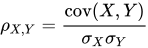
ค่าสัมประสิทธิ์สหสัมพันธ์แบบเพียร์สันระหว่างตัวแปรสุ่มสองตัวและถูกกำหนดให้เป็น
ที่ไหน
- คือค่าความแปรปรวนร่วม
- คือค่าเบี่ยงเบนมาตรฐานของ
- คือค่าเบี่ยงเบนมาตรฐานของ .


ตัวส่วนสามารถเขียนได้อีกแบบว่าซึ่งก็คือค่าเฉลี่ยเรขาคณิตของค่าความแปรปรวน

ดังนั้นเราจึงเห็นว่าสัมประสิทธิ์สหสัมพันธ์เป็นรูปแบบมาตรฐานของความแปรปรวนร่วม โดยจะมีค่าอยู่ระหว่าง เสมอและและไม่มีหน่วย (ต่างจากค่าความแปรปรวนร่วม)


ค่าสัมประสิทธิ์สหสัมพันธ์มักใช้สัญลักษณ์rและมักถูกรายงานในงานวิจัยทางวิทยาศาสตร์
การวิเคราะห์ส่วนประกอบหลัก
เมทริกซ์ความแปรปรวนร่วมถูกนำมาใช้ในการวิเคราะห์องค์ประกอบหลักเพื่อลดมิติของคุณลักษณะในการประมวลผลข้อมูลเบื้องต้น องค์ประกอบหลักคือมิติที่อธิบายความแปรปรวนส่วนใหญ่ในข้อมูล การประยุกต์ใช้ที่รู้จักกันดีคือในด้านสติปัญญา โดยสร้างปัจจัย gขึ้นมา อีกตัวอย่างหนึ่งคือด้านบุคลิกภาพ โดยแบบจำลองต่างๆ เช่นแบบจำลองห้าปัจจัยได้มาจากการวิเคราะห์องค์ประกอบหลัก