ในทางคณิตศาสตร์ สัญกรณ์ลูกศรขึ้นของ Knuth เป็นวิธีการเขียนสัญกรณ์สำหรับจำนวนเต็มขนาด ใหญ่มาก ซึ่ง Donald Knuth นำเสนอในปี 1976 [ 1 ]
ในบทความปี 1947 ของเขา[ 2 ] RL Goodstein ได้แนะนำลำดับการดำเนินการเฉพาะที่ปัจจุบันเรียกว่าไฮเปอร์โอเปอเรชัน tetration , pentation เป็นต้น สำหรับการดำเนินการที่ขยายออกไปนอกเหนือจากการยกกำลัง ลำดับเริ่มต้นด้วยการดำเนินการเอกภาค ( ฟังก์ชันตัวสืบทอด ที่มีn = 0) และดำเนินต่อไปด้วยการดำเนินการทวิภาค ของการบวก ( n = 1), การคูณ ( n = 2), การยกกำลัง ( n = 3), tetration ( n = 4) เป็นต้น มีการใช้ สัญกรณ์ต่างๆ เพื่อแสดงไฮเปอร์โอเปอเรชัน สัญกรณ์หนึ่งดังกล่าวคือชม n ( เอ , ข ) {\displaystyle H_{n}(a,b)} ↑ {\displaystyle \uparrow }
ลูกศรเดี่ยว↑ {\displaystyle \uparrow } การยกกำลัง (การคูณซ้ำๆ)2 ↑ 4 = ชม 3 ( 2 , 4 ) = 2 × ( 2 × ( 2 × 2 ) ) = 2 4 = 16 {\displaystyle 2\uparrow 4=H_{3}(2,4)=2\times (2\times (2\times 2))=2^{4}=16} ลูกศรคู่↑ ↑ {\displaystyle \uparrow \uparrow } tetration )2 ↑ ↑ 4 = ชม 4 ( 2 , 4 ) = 2 ↑ ( 2 ↑ ( 2 ↑ 2 ) ) = 2 2 2 2 = 2 16 = 65 , 536 {\displaystyle 2\uparrow \uparrow 4=H_{4}(2,4)=2\uparrow (2\uparrow (2\uparrow 2))=2^{2^{2^{2}}}=2^{16}=65,536} ลูกศรสามอัน↑ ↑ ↑ {\displaystyle \uparrow \uparrow \uparrow } 2 ↑ ↑ ↑ 4 = ชม 5 ( 2 , 4 ) = 2 ↑ ↑ ( 2 ↑ ↑ ( 2 ↑ ↑ 2 ) ) = 2 ↑ ↑ ( 2 ↑ ↑ ( 2 ↑ 2 ) ) = 2 ↑ ↑ ( 2 ↑ ↑ 4 ) = 2 ↑ ( 2 ↑ ( 2 ↑ ⋯ ) ) ⏟ = 2 2 ⋯ 2 ⏟ 2 ↑ ↑ 4 สำเนาของ 2 65,536 เลข 2 {\displaystyle {\begin{aligned}2\uparrow \uparrow \uparrow 4&=H_{5}(2,4)\\&=2\uparrow \uparrow (2\uparrow \uparrow (2\uparrow \uparrow 2))\\&=2\uparrow \uparrow (2\uparrow \uparrow (2\uparrow 2))\\&=2\uparrow \uparrow (2\uparrow \uparrow 4)\\&=\underbrace {2\uparrow (2\uparrow (2\uparrow \cdots ))} \;=\;\underbrace {\;2^{2^{\cdots ^{2}}}} \\&\;\;\;\;\;2\uparrow \uparrow 4{\text{ copies of }}2\;\;\;\;\;{\text{65,536 2's}}\\\end{aligned}}} นิยามทั่วไปของสัญลักษณ์ลูกศรชี้ขึ้นมีดังนี้ (สำหรับเอ ≥ 0 , n ≥ 1 , ข ≥ 0 {\displaystyle a\geq 0,n\geq 1,b\geq 0} เอ ↑ n ข = ชม n + 2 ( เอ , ข ) = เอ [ n + 2 ] ข . {\displaystyle a\uparrow ^{n}b=H_{n+2}(a,b)=a[n+2]b.} ↑ n {\displaystyle \uparrow ^{n}} n ตัว ตัวอย่างเช่น 2 ↑ ↑ ↑ ↑ 3 = 2 ↑ 4 3 , {\displaystyle 2\uparrow \uparrow \uparrow \uparrow 3=2\uparrow ^{4}3,}
การแนะนำ การดำเนิน การขั้นสูง (Hyperoperations) เป็นการ ต่อยอดการดำเนินการ ทางคณิตศาสตร์ ของการบวก และการคูณ อย่างเป็นธรรมชาติดังต่อไปนี้
การบวกด้วยจำนวนธรรมชาติ เรียกว่า การเพิ่มค่าแบบวนซ้ำ:
ชม 1 ( เอ , ข ) = เอ + ข = เอ + 1 + 1 + ⋯ + 1 ⏟ ข สำเนาของ 1 {\displaystyle {\begin{matrix}H_{1}(a,b)=a+b=&a+\underbrace {1+1+\dots +1} \\&b{\mbox{ copies of }}1\end{matrix}}} การคูณด้วยจำนวนธรรมชาติถูกนิยามว่าเป็นการบวกซ้ำๆ:
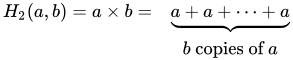
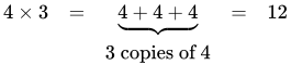
ชม 2 ( เอ , ข ) = เอ × ข = เอ + เอ + ⋯ + เอ ⏟ ข สำเนาของ เอ {\displaystyle {\begin{matrix}H_{2}(a,b)=a\times b=&\underbrace {a+a+\dots +a} \\&b{\mbox{ copies of }}a\end{matrix}}} ตัวอย่างเช่น,
4 × 3 = 4 + 4 + 4 ⏟ = 12 3 สำเนาของ 4 {\displaystyle {\begin{matrix}4\times 3&=&\underbrace {4+4+4} &=&12\\&&3{\mbox{ copies of }}4\end{matrix}}} การยกกำลัง สำหรับพลังงานธรรมชาติข {\displaystyle b}
เอ ↑ ข = ชม 3 ( เอ , ข ) = เอ ข = เอ × เอ × ⋯ × เอ ⏟ ข สำเนาของ เอ {\displaystyle {\begin{matrix}a\uparrow b=H_{3}(a,b)=a^{b}=&\underbrace {a\times a\times \dots \times a} \\&b{\mbox{ สำเนาของ }}a\end{matrix}}} ตัวอย่างเช่น,
4 ↑ 3 = 4 3 = 4 × 4 × 4 ⏟ = 64 3 สำเนาของ 4 {\displaystyle {\begin{matrix}4\uparrow 3=4^{3}=&\underbrace {4\times 4\times 4} &=&64\\&3{\mbox{ copies of }}4\end{matrix}}} Tetration ถูกนิยามว่าเป็นการยกกำลังซ้ำๆ ซึ่ง Knuth ใช้สัญลักษณ์ "ลูกศรคู่" แทน:
เอ ↑ ↑ ข = ชม 4 ( เอ , ข ) = เอ เอ . . . เอ ⏟ = เอ ↑ ( เอ ↑ ( ⋯ ↑ เอ ) ) ⏟ ข สำเนาของ เอ ข สำเนาของ เอ {\displaystyle {\begin{matrix}a\uparrow \uparrow b=H_{4}(a,b)=&\underbrace {a^{a^{{}^{.\,^{.\,^{.\,^{a}}}}}}} &=&\underbrace {a\uparrow (a\uparrow (\cdots \uparrow a))} \\&b{\mbox{ สำเนาของ }}a&&b{\mbox{ สำเนาของ }}a\end{matrix}}} ตัวอย่างเช่น,
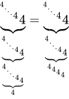
4 ↑ ↑ 3 = 4 4 4 ⏟ = 4 ↑ ( 4 ↑ 4 ) ⏟ = 4 256 3 สำเนาของ 4 3 สำเนาของ 4 {\displaystyle {\begin{matrix}4\uparrow \uparrow 3=&\underbrace {4^{4^{4}}} &=&\underbrace {4\uparrow (4\uparrow 4)} &=&4^{256}&&\\&3{\mbox{ สำเนาของ }}4&&3{\mbox{ สำเนาของ }}4\end{matrix}}} นิพจน์จะถูกประเมินจากขวาไปซ้าย เนื่องจากตัวดำเนินการถูกกำหนดให้เป็นแบบเชื่อมโยงทาง ขวา
ตามคำจำกัดความนี้
3 ↑ ↑ 2 = 3 3 = 27 {\displaystyle 3\uparrow \uparrow 2=3^{3}=27} 3 ↑ ↑ 3 = 3 3 3 = 3 27 = 7 , 625 , 597 , 484 , 987 {\displaystyle 3\uparrow \uparrow 3=3^{3^{3}}=3^{27}=7,625,597,484,987} 3 ↑ ↑ 4 = 3 3 3 3 = 3 3 27 = 3 7625597484987 {\displaystyle 3\uparrow \uparrow 4=3^{3^{3^{3}}}=3^{3^{27}}=3^{7625597484987}} 3 ↑ ↑ 5 = 3 3 3 3 3 = 3 3 3 27 = 3 3 7625597484987 {\displaystyle 3\uparrow \uparrow 5=3^{3^{3^{3^{3}}}}=3^{3^{3^{27}}}=3^{3^{7625597484987}}} เป็นต้น สิ่งนี้ทำให้ได้ตัวเลขที่ค่อนข้างใหญ่แล้ว แต่ลำดับของไฮเปอร์โอเปอเรเตอร์ยังไม่จบเพียงเท่านี้ เพนเทชัน ซึ่งนิยามว่าเป็นเทเทชันแบบวนซ้ำ จะถูกแทนด้วย "ลูกศรสามหัว":
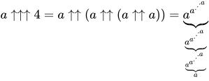
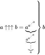
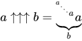
เอ ↑ ↑ ↑ ข = ชม 5 ( เอ , ข ) = เอ ↑ ↑ ( เอ ↑ ↑ ( ⋯ ↑ ↑ เอ ) ) ⏟ ข สำเนาของ เอ {\displaystyle {\begin{matrix}a\uparrow \uparrow \uparrow b=H_{5}(a,b)=&\underbrace {a_{}\uparrow \uparrow (a\uparrow \uparrow (\cdots \uparrow \uparrow a))} \\&b{\mbox{ copies of }}a\end{matrix}}} การคูณแบบเฮกเซชัน ซึ่งนิยามว่าเป็นการคูณแบบเพนเทชันซ้ำๆ นั้น แสดงด้วย "ลูกศรสี่แฉก":
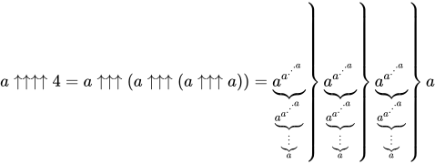
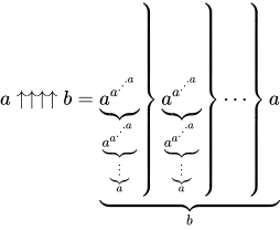
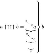
เอ ↑ ↑ ↑ ↑ ข = ชม 6 ( เอ , ข ) = เอ ↑ ↑ ↑ ( เอ ↑ ↑ ↑ ( ⋯ ↑ ↑ ↑ เอ ) ) ⏟ ข สำเนาของ เอ {\displaystyle {\begin{matrix}a\uparrow \uparrow \uparrow \uparrow b=H_{6}(a,b)=&\underbrace {a_{}\uparrow \uparrow \uparrow (a\uparrow \uparrow \uparrow (\cdots \uparrow \uparrow \uparrow a))} \\&b{\mbox{ copies of }}a\end{matrix}}} และอื่นๆ โดยทั่วไปแล้วกฎก็คือว่าn {\displaystyle n} n − 1 {\displaystyle n-1}
เอ ↑ ↑ ⋯ ↑ ⏟ n ข = เอ ↑ ⋯ ↑ ⏟ n − 1 ( เอ ↑ ⋯ ↑ ⏟ n − 1 ( ⋯ ↑ ⋯ ↑ ⏟ n − 1 เอ ) ) ⏟ ข สำเนาของ เอ {\displaystyle {\begin{matrix}a\ \underbrace {\uparrow _{}\uparrow \!\!\cdots \!\!\uparrow } _{n}\ b=\underbrace {a\ \underbrace {\uparrow \!\!\cdots \!\!\uparrow } _{n-1}\ (a\ \underbrace {\uparrow _{}\!\!\cdots \!\!\uparrow } _{n-1}\ (\cdots \ \underbrace {\uparrow _{}\!\!\cdots \!\!\uparrow } _{n-1}\ a))} _{b{\text{ copies of }}a}\end{matrix}}} ตัวอย่าง:
3 ↑ ↑ ↑ 2 = 3 ↑ ↑ 3 = 3 3 3 = 3 27 = 7 , 625 , 597 , 484 , 987 {\displaystyle 3\uparrow \uparrow \uparrow 2=3\uparrow \uparrow 3=3^{3^{3}}=3^{27}=7,625,597,484,987} 3 ↑ ↑ ↑ 3 = 3 ↑ ↑ ( 3 ↑ ↑ 3 ) = 3 ↑ ↑ ( 3 ↑ 3 ↑ 3 ) = 3 ↑ 3 ↑ ⋯ ↑ 3 ⏟ 3 ↑ 3 ↑ 3 สำเนาของ 3 = 3 ↑ 3 ↑ ⋯ ↑ 3 ⏟ 7,625,597,484,987 ชุดของ 3 = 3 3 3 3 ⋅ ⋅ ⋅ ⋅ 3 ⏟ 7,625,597,484,987 ชุดของ 3 {\displaystyle {\begin{aligned}3\uparrow \uparrow \uparrow 3&=3\uparrow \uparrow (3\uparrow \uparrow 3)\\&=3\uparrow \uparrow (3\uparrow 3\uparrow 3)\\&={\begin{matrix}\underbrace {3\uparrow 3\uparrow \cdots \uparrow 3} \\3\uparrow 3\uparrow 3{\mbox{ copies of }}3\end{matrix}}\\&={\begin{matrix}\underbrace {3\uparrow 3\uparrow \cdots \uparrow 3} \\{\mbox{7,625,597,484,987 copies of 3}}\end{matrix}}\\&={\begin{matrix}\underbrace {3^{3^{3^{3^{\cdot ^{\cdot ^{\cdot ^{\cdot ^{3}}}}}}}}} \\{\mbox{7,625,597,484,987 copies of 3}}\end{matrix}}\end{aligned}}}
การสรุปโดยทั่วไป บางตัวเลขมีขนาดใหญ่มากจนการใช้ลูกศรหลายตัวในสัญกรณ์ลูกศรขึ้นของ Knuth กลายเป็นเรื่องยุ่งยากเกินไป ดังนั้นจึงต้องใช้ตัวดำเนินการลูกศร n ตัว ↑ n {\displaystyle \uparrow ^{n}} ตัวดำเนินการไฮ เปอร์
Some numbers are so large that even that notation is not sufficient. The Conway chained arrow notation can then be used: a chain of three elements is equivalent with the other notations, but a chain of four or more is even more powerful.
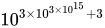
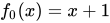
a ↑ n b = a [ n + 2 ] b = a → b → n (Knuth) (hyperoperation) (Conway) {\displaystyle {\begin{matrix}a\uparrow ^{n}b&=&a[n+2]b&=&a\to b\to n\\{\text{(Knuth)}}&&{\text{(hyperoperation)}}&&{\text{(Conway)}}\end{matrix}}} 6 ↑↑ 4 = 6 6 . . . 6 ⏟ 4 {\displaystyle 6\uparrow \uparrow 4=\underbrace {6^{6^{.^{.^{.^{6}}}}}} _{4}} 6 ↑↑ 4 = 6 6 6 6 = 6 6 46 , 656 {\displaystyle 6\uparrow \uparrow 4=6^{6^{6^{6}}}=6^{6^{46,656}}} 6 6 . . . 6 ⏟ 4 {\displaystyle \underbrace {6^{6^{.^{.^{.^{6}}}}}} _{4}} 10 ↑ ( 3 × 10 ↑ ( 3 × 10 ↑ 15 ) + 3 ) = 100000 … 000 ⏟ 300000 … 003 ⏟ 300000 … 000 ⏟ 15 {\displaystyle 10\uparrow (3\times 10\uparrow (3\times 10\uparrow 15)+3)=\underbrace {100000\ldots 000} _{\underbrace {300000\ldots 003} _{\underbrace {300000\ldots 000} _{15}}}} 10 3 × 10 3 × 10 15 + 3 {\displaystyle 10^{3\times 10^{3\times 10^{15}}+3}} Even faster-growing functions can be categorized using an ordinal analysis called the fast-growing hierarchy . The fast-growing hierarchy uses successive function iteration and diagonalization to systematically create faster-growing functions from some base function f ( x ) {\displaystyle f(x)} f 0 ( x ) = x + 1 {\displaystyle f_{0}(x)=x+1} f 2 ( x ) {\displaystyle f_{2}(x)} f 3 ( x ) {\displaystyle f_{3}(x)} f ω ( x ) {\displaystyle f_{\omega }(x)} Ackermann function , f ω + 1 ( x ) {\displaystyle f_{\omega +1}(x)} Graham's number , and f ω 2 ( x ) {\displaystyle f_{\omega ^{2}}(x)}
These functions are all computable. Even faster computable functions, such as the Goodstein sequence and the TREE sequence require the usage of large ordinals, may occur in certain combinatorical and proof-theoretic contexts. There exist functions which grow uncomputably fast, such as the Busy Beaver , which by their very nature will be completely out of reach from any up-arrow, or even any ordinal-based analysis.
Definition Without reference to hyperoperation the up-arrow operators can be formally defined by
a ↑ n b = { a b , if n = 1 ; 1 , if n > 1 and b = 0 ; a ↑ n − 1 ( a ↑ n ( b − 1 ) ) , otherwise {\displaystyle a\uparrow ^{n}b={\begin{cases}a^{b},&{\text{if }}n=1;\\1,&{\text{if }}n>1{\text{ and }}b=0;\\a\uparrow ^{n-1}(a\uparrow ^{n}(b-1)),&{\text{otherwise }}\end{cases}}} for all integers a , b , n {\displaystyle a,b,n} a ≥ 0 , n ≥ 1 , b ≥ 0 {\displaystyle a\geq 0,n\geq 1,b\geq 0} [ nb 1]
This definition uses exponentiation ( a ↑ 1 b = a ↑ b = a b ) {\displaystyle (a\uparrow ^{1}b=a\uparrow b=a^{b})} tetration ( a ↑ 2 b = a ↑↑ b ) {\displaystyle (a\uparrow ^{2}b=a\uparrow \uparrow b)} hyperoperation sequence except it omits the three more basic operations of succession , addition and multiplication .
One can alternatively choose multiplication ( a ↑ 0 b = a × b ) {\displaystyle (a\uparrow ^{0}b=a\times b)} exponentiation becomes repeated multiplication. The formal definition would be
a ↑ n b = { a × b , if n = 0 ; 1 , if n > 0 and b = 0 ; a ↑ n − 1 ( a ↑ n ( b − 1 ) ) , otherwise {\displaystyle a\uparrow ^{n}b={\begin{cases}a\times b,&{\text{if }}n=0;\\1,&{\text{if }}n>0{\text{ and }}b=0;\\a\uparrow ^{n-1}(a\uparrow ^{n}(b-1)),&{\text{otherwise }}\end{cases}}} for all integers a , b , n {\displaystyle a,b,n} a ≥ 0 , n ≥ 0 , b ≥ 0 {\displaystyle a\geq 0,n\geq 0,b\geq 0}
Note, however, that Knuth did not define the "nil-arrow" (↑ 0 {\displaystyle \uparrow ^{0}}
H n ( a , b ) = a [ n ] b = a ↑ n − 2 b for n ≥ 0. {\displaystyle H_{n}(a,b)=a[n]b=a\uparrow ^{n-2}b{\text{ for }}n\geq 0.} The up-arrow operation is a right-associative operation , that is, a ↑ b ↑ c {\displaystyle a\uparrow b\uparrow c} a ↑ ( b ↑ c ) {\displaystyle a\uparrow (b\uparrow c)} ( a ↑ b ) ↑ c {\displaystyle (a\uparrow b)\uparrow c}
ตารางค่าต่างๆ
n b การคำนวณ0 ↑ n ข = ชม n + 2 ( 0 , ข ) = 0 [ n + 2 ] ข {\displaystyle 0\uparrow ^{n}b=H_{n+2}(0,b)=0[n+2]b}
0 เมื่อn = 0 [ nb 2 ] 1 เมื่อn = 1 และb = 0 [ nb 1 ] [ nb 3 ] 0 เมื่อn = 1 และb > 0 [ nb 1 ] [ nb 3 ] 1 เมื่อn > 1 และb เป็นจำนวนคู่ (รวมถึง 0) 0 เมื่อn > 1 และb เป็นจำนวนคี่
n b การคำนวณ2 ↑ n ข {\displaystyle 2\uparrow ^{n}b} 2 ข {\displaystyle 2^{b}}
ตารางนี้เหมือนกับตารางของฟังก์ชัน Ackermann ทุก ประการ ยกเว้นการเลื่อนตำแหน่งในn {\displaystyle n} ข {\displaystyle b}
↑ n b เราวางตัวเลข3 ข {\displaystyle 3^{b}}
ค่านิยมของ3 ↑ n ข = {\displaystyle 3\uparrow ^{n}b={}} ชม n + 2 ( 3 , ข ) = {\displaystyle H_{n+2}(3,b)={}} 3 [ n + 2 ] ข = {\displaystyle 3[n+2]b={}} 3 → b → n ข
n
1 2 3 4 5 สูตร 1 3 9 27 81 243 3 ข {\displaystyle 3^{b}} 2 3 27 7,625,597,484,987 3 7625597484987 ≈ 1.25801 × 10 3638334640024 {\displaystyle 3^{7625597484987}\approx 1.25801\times 10^{3638334640024}} 3 3 7625597484987 ≈ 10 6.00225 × 10 3638334640023 {\displaystyle 3^{3^{7625597484987}}\approx 10^{6.00225\times 10^{3638334640023}}} 3 ↑ ↑ ข {\displaystyle 3\uparrow \uparrow b} 3 3 7,625,597,484,987 7625597484987 3 {\displaystyle {}^{7625597484987}{3}} 7625597484987 3 3 {\displaystyle {}^{{}^{7625597484987}{3}}{3}} 7625597484987 3 3 3 {\displaystyle {}^{{}^{{}^{7625597484987}{3}}{3}}{3}} 3 ↑ ↑ ↑ ข {\displaystyle 3\uparrow \uparrow \uparrow b} 4 3 3 ↑ ↑ ↑ 7625597484987 3 {\displaystyle 3\uparrow \uparrow \uparrow {}^{7625597484987}{3}} 3 ↑ ↑ ↑ ( 3 ↑ ↑ ↑ 7625597484987 3 ) {\displaystyle 3\uparrow \uparrow \uparrow (3\uparrow \uparrow \uparrow {}^{7625597484987}{3})} 3 ↑ ↑ ↑ ( 3 ↑ ↑ ↑ ( 3 ↑ ↑ ↑ 7625597484987 3 ) ) {\displaystyle 3\uparrow \uparrow \uparrow (3\uparrow \uparrow \uparrow (3\uparrow \uparrow \uparrow {}^{7625597484987}{3}))} 3 ↑ ↑ ↑ ( 3 ↑ ↑ ↑ ( 3 ↑ ↑ ↑ ( 3 ↑ ↑ ↑ 7625597484987 3 ) ) ) {\displaystyle 3\uparrow \uparrow \uparrow (3\uparrow \uparrow \uparrow (3\uparrow \uparrow \uparrow (3\uparrow \uparrow \uparrow {}^{7625597484987}{3})))} 3 ↑ ↑ ↑ ↑ ข {\displaystyle 3\uparrow \uparrow \uparrow \uparrow b}
↑ n b เราวางตัวเลข4 ข {\displaystyle 4^{b}}
↑ n b เราวางตัวเลข10 ข {\displaystyle 10^{b}}
ค่านิยมของ10 ↑ n ข = {\displaystyle 10\uparrow ^{n}b={}} ชม n + 2 ( 10 , ข ) = {\displaystyle H_{n+2}(10,b)={}} 10 [ n + 2 ] ข = {\displaystyle 10[n+2]b={}} 10 → b → n ข
n
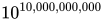
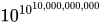
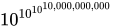
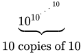
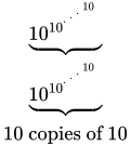
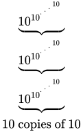
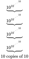
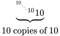
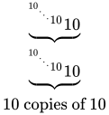
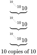
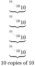
1 2 3 4 5 สูตร 1 10 100 1,000 10,000 100,000 10 ข {\displaystyle 10^{b}} 2 10 10,000,000,000 10 10 , 000 , 000 , 000 {\displaystyle 10^{10,000,000,000}} 10 10 10 , 000 , 000 , 000 {\displaystyle 10^{10^{10,000,000,000}}} 10 10 10 10 , 000 , 000 , 000 {\displaystyle 10^{10^{10^{10,000,000,000}}}} 10 ↑ ↑ ข {\displaystyle 10\uparrow \uparrow b} 3 10 10 10 . . . 10 ⏟ 10 สำเนาของ 10 {\displaystyle {\begin{matrix}\underbrace {10_{}^{10^{{}^{.\,^{.\,^{.\,^{10}}}}}}} \\10{\mbox{ copies of }}10\end{matrix}}} 10 10 . . . 10 ⏟ 10 10 . . . 10 ⏟ 10 สำเนาของ 10 {\displaystyle {\begin{matrix}\underbrace {10_{}^{10^{{}^{.\,^{.\,^{.\,^{10}}}}}}} \\\underbrace {10_{}^{10^{{}^{.\,^{.\,^{.\,^{10}}}}}}} \\10{\mbox{ copies of }}10\end{matrix}}} 10 10 . . . 10 ⏟ 10 10 . . . 10 ⏟ 10 10 . . . 10 ⏟ 10 สำเนาของ 10 {\displaystyle {\begin{matrix}\underbrace {10_{}^{10^{{}^{.\,^{.\,^{.\,^{10}}}}}}} \\\underbrace {10_{}^{10^{{}^{.\,^{.\,^{.\,^{10}}}}}}} \\\underbrace {10_{}^{10^{{}^{.\,^{.\,^{.\,^{10}}}}}}} \\10{\mbox{ copies of }}10\end{matrix}}} 10 10 . . . 10 ⏟ 10 10 . . . 10 ⏟ 10 10 . . . 10 ⏟ 10 10 . . . 10 ⏟ 10 สำเนาของ 10 {\displaystyle {\begin{matrix}\underbrace {10_{}^{10^{{}^{.\,^{.\,^{.\,^{10}}}}}}} \\\underbrace {10_{}^{10^{{}^{.\,^{.\,^{.\,^{10}}}}}}} \\\underbrace {10_{}^{10^{{}^{.\,^{.\,^{.\,^{10}}}}}}} \\\underbrace {10_{}^{10^{{}^{.\,^{.\,^{.\,^{10}}}}}}} \\10{\mbox{ copies of }}10\end{matrix}}} 10 ↑ ↑ ↑ ข {\displaystyle 10\uparrow \uparrow \uparrow b} 4 10 10 . . . 10 10 ⏟ 10 สำเนาของ 10 {\displaystyle {\begin{matrix}\underbrace {^{^{^{^{^{10}.}.}.}10}10} \\10{\mbox{ copies of }}10\end{matrix}}} 10 . . . 10 10 ⏟ 10 . . . 10 10 ⏟ 10 สำเนาของ 10 {\displaystyle {\begin{matrix}\underbrace {^{^{^{^{^{10}.}.}.}10}10} \\\underbrace {^{^{^{^{^{10}.}.}.}10}10} \\10{\mbox{ copies of }}10\end{matrix}}} 10 . . . 10 10 ⏟ 10 . . . 10 10 ⏟ 10 . . . 10 10 ⏟ 10 สำเนาของ 10 {\displaystyle {\begin{matrix}\underbrace {^{^{^{^{^{10}.}.}.}10}10} \\\underbrace {^{^{^{^{^{10}.}.}.}10}10} \\\underbrace {^{^{^{^{^{10}.}.}.}10}10} \\10{\mbox{ copies of }}10\end{matrix}}} 10 . . . 10 10 ⏟ 10 . . . 10 10 ⏟ 10 . . . 10 10 ⏟ 10 . . . 10 10 ⏟ 10 สำเนาของ 10 {\displaystyle {\begin{matrix}\underbrace {^{^{^{^{^{10}.}.}.}10}10} \\\underbrace {^{^{^{^{^{10}.}.}.}10}10} \\\underbrace {^{^{^{^{^{10}.}.}.}10}10} \\\underbrace {^{^{^{^{^{10}.}.}.}10}10} \\10{\mbox{ copies of }}10\end{matrix}}} 10 ↑ ↑ ↑ ↑ ข {\displaystyle 10\uparrow \uparrow \uparrow \uparrow b}
สำหรับ 2 ≤ b ≤ 9 ลำดับตัวเลขของจำนวนต่างๆ10 ↑ n ข {\displaystyle 10\uparrow ^{n}b} ลำดับพจนานุกรม โดยที่n เป็นตัวเลขที่มีค่ามากที่สุด ดังนั้นสำหรับตัวเลขใน 8 คอลัมน์นี้ ลำดับตัวเลขจึงเรียงตามบรรทัดต่อบรรทัด หลักการเดียวกันนี้ใช้ได้กับตัวเลขใน 97 คอลัมน์ โดยที่ 3 ≤ b ≤ 99 และหากเราเริ่มต้นจากn = 1 ก็จะใช้ได้กับ 3 ≤ b ≤ 9,999,999,999 เช่นกัน
หมายเหตุ 1 2 3 สำหรับรายละเอียดเพิ่มเติม โปรดดูที่ เลขยกกำลังของ ศูนย์ ↑ โปรดจำไว้ว่า Knuth ไม่ได้นิยามตัวดำเนินการนี้↑ 0 {\displaystyle \uparrow ^{0}} 1 2 สำหรับรายละเอียดเพิ่มเติม โปรดดูยกกำลังศูนย์ 








![{\displaystyle a\uparrow ^{n}b=H_{n+2}(a,b)=a[n+2]b.}](https://wikimedia.org/api/rest_v1/media/math/render/svg/85c46ffdf75f03948d485eeffeea3486354eb211)
























![{\displaystyle {\begin{matrix}a\uparrow ^{n}b&=&a[n+2]b&=&a\to b\to n\\{\text{(Knuth)}}&&{\text{(hyperoperation)}}&&{\text{(Conway)}}\end{matrix}}}](https://wikimedia.org/api/rest_v1/media/math/render/svg/2a66f541418af751ad278b277ed9a18964c4a96a)













![{\displaystyle H_{n}(a,b)=a[n]b=a\uparrow ^{n-2}b{\text{ สำหรับ }}n\geq 0.}](https://wikimedia.org/api/rest_v1/media/math/render/svg/013f5aded05b23ab8552efd77dca57c4694d8b1e)


![{\displaystyle 0\uparrow ^{n}b=H_{n+2}(0,b)=0[n+2]b}](https://wikimedia.org/api/rest_v1/media/math/render/svg/c74b3c65305086a3ffe141df38df0ae9061806ef)


![{\displaystyle 2[n+2]b={}}](https://wikimedia.org/api/rest_v1/media/math/render/svg/bf3495c599bba92d3e9eebcdc301fee377b5e88d)


![{\displaystyle 3[n+2]b={}}](https://wikimedia.org/api/rest_v1/media/math/render/svg/08394e1a60c724f5ea6cddbae1335bbfd3cd990b)


![{\displaystyle 4[n+2]b={}}](https://wikimedia.org/api/rest_v1/media/math/render/svg/970000c453179f61f91e0856dc6ff81baa1cd171)


![{\displaystyle 10[n+2]b={}}](https://wikimedia.org/api/rest_v1/media/math/render/svg/5a5269a50acca4e5ee9f39dbc78cacab87f4a1c6)