ในทางคณิตศาสตร์ฟังก์ชันไฮเปอร์โบลิกเป็นอนาล็อกของฟังก์ชันตรีโกโนเมตริก ทั่วไป แต่กำหนดโดยใช้ไฮเปอร์โบลาแทนวงกลมเช่นเดียวกับที่จุด(cos t , sin t )ก่อตัวเป็นวงกลมที่มีรัศมีหนึ่งหน่วยจุด(cosh t , sinh t )ก่อตัวเป็นครึ่งขวาของไฮเปอร์โบลาหน่วยในทำนองเดียวกันกับที่อนุพันธ์ของsin( t )และcos( t )คือcos( t )และ –sin ( t )อนุพันธ์ของsinh( t )และcosh( t )คือcosh( t )และsinh( t )

ฟังก์ชันไฮเปอร์โบลิกใช้เพื่อแสดงมุมขนานในเรขาคณิตไฮเปอร์โบลิก นอกจากนี้ยัง ใช้เพื่อแสดงการเพิ่มความเร็วแบบลอเรนซ์เป็นการหมุนแบบไฮเปอร์โบลิกในทฤษฎีสัมพัทธภาพพิเศษ และยังพบได้ในคำตอบของ สมการเชิงอนุพันธ์เชิงเส้นหลาย สมการ (เช่น สมการที่กำหนดเส้นโค้งแคทเทนารี ) สมการกำลังสามและสมการลาปลาสในพิกัดคาร์ทีเซียนสมการลาปลาสมีความสำคัญในหลายสาขาของฟิสิกส์รวมถึงทฤษฎีแม่เหล็กไฟฟ้าการถ่ายเทความร้อนและพลศาสตร์ของไหล

ฟังก์ชันไฮเปอร์โบลิกพื้นฐานคือ: ^{[ 1 ]}

• ไฮเปอร์โบลิกไซน์ " sinh " ( / ˈ s ə ŋ , ˈ s ɪ n tʃ , ˈ ʃ aɪ n / ) , ^{[ 2 ]}
• โคไซน์ไฮเปอร์โบลิก " cosh " ( / ˈ k ɒ ʃ , ˈ k oʊ ʃ / ), ^{[ 3 ]}

ซึ่งได้มาจาก: ^{[ 4 ]}

• แทนเจนต์ซึ่งเกินความจริง " tanh " ( / ˈ t æ ŋ , ˈ t æ n tʃ , ˈ θ æ n / ), ^{[ 5 ]}
• โคแทนเจนต์ไฮเปอร์โบลิก " coth " ( / ˈ k ɒ θ , ˈ k oʊ θ / ), ^{[ 6 ] [ 7 ]}
• ไฮเปอร์โบลิกซีแคนต์ " sech " ( / ˈ s ɛ tʃ , ˈ ʃ ɛ k / ), ^{[ 8 ]}
• โคซีแคนต์ซึ่งเกินความจริง " csch " หรือ " cosech " ( / ˈ k oʊ s ɛ tʃ , ˈ k oʊ ʃ ɛ k / ^{[ 3 ]} )

ซึ่งสอดคล้องกับฟังก์ชันตรีโกณมิติที่ได้มา

ฟังก์ชันไฮเปอร์โบลิกผกผันได้แก่:

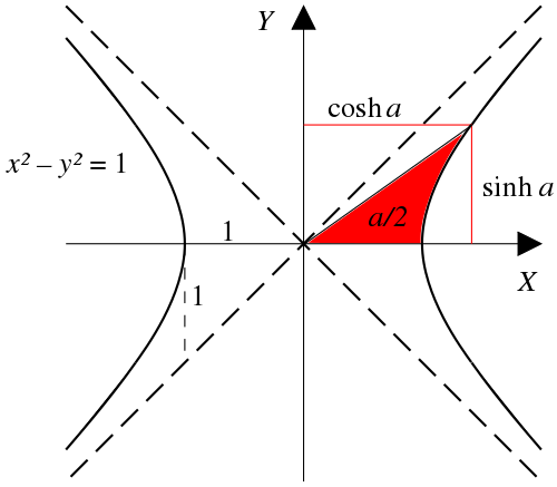
• ไซน์ไฮเปอร์โบลิกผกผัน " arsinh " (หรือเขียนแทนด้วย " sinh ⁻¹ ", " asinh " หรือบางครั้ง " arcsinh ") ^{[ 9 ] [ 10 ] [ 11 ]}
• โคไซน์ไฮเปอร์โบลิกผกผัน " arcosh " (หรือเขียนแทนด้วย " cosh ⁻¹ ", " acosh " หรือบางครั้ง " arccosh ")
• แทนเจนต์ไฮเปอร์โบลิกผกผัน " artanh " (หรือเขียนแทนด้วย " tanh ⁻¹ ", " atanh " หรือบางครั้ง " arctanh ")
• โคแทนเจนต์ไฮเปอร์โบลิกผกผัน " arcoth " (หรือเขียนแทนด้วย " coth ⁻¹ ", " acoth " หรือบางครั้ง " arccoth ")
• ตัวผกผันไฮเปอร์โบลิกซีแคนต์ " arsech " (หรือเขียนแทนด้วย " sech ⁻¹ ", " asech " หรือบางครั้ง " arcsech ")
• โคเซแคนต์ไฮเปอร์โบลิกผกผัน " arcsch " (หรือเขียนแทนด้วย " arcosech ", " csch ⁻¹ ", " cosech ⁻¹ ", " acsch ", " acosech " หรือบางครั้งอาจเขียนว่า " arccsch " หรือ " arccosech ")

ฟังก์ชันไฮเปอร์โบลิกมีตัวแปรที่เรียกว่ามุมไฮเปอร์โบลิกขนาดของมุมไฮเปอร์โบลิกคือพื้นที่ของส่วนโค้งไฮเปอร์โบลิกที่ ลาก ผ่านเส้น ตรง xy = 1ฟังก์ชันไฮเปอร์โบลิกอาจถูกกำหนดโดยใช้ด้านประกอบมุมฉากของสามเหลี่ยมมุมฉากที่ครอบคลุมส่วนโค้งนี้

ในการวิเคราะห์เชิงซ้อนฟังก์ชันไฮเปอร์โบลิกเกิดขึ้นเมื่อนำฟังก์ชันไซน์และโคไซน์ธรรมดาไปใช้กับมุมจินตนาการ ฟังก์ชันไซน์ไฮเปอร์โบลิกและฟังก์ชันโคไซน์ไฮเปอร์โบลิกเป็นฟังก์ชันเอนไทร์ดังนั้น ฟังก์ชันไฮเปอร์โบลิกอื่นๆ จึงเป็นฟังก์ชันเมโรเมอร์ฟิกในระนาบเชิงซ้อนทั้งหมด

ตามทฤษฎีบทของ Lindemann–Weierstrassฟังก์ชันไฮเปอร์โบลิกมีค่าอดิศัย สำหรับทุก ค่าพีชคณิตที่ไม่เป็นศูนย์ของอาร์กิวเมนต์^{[ 12 ]}

การคำนวณครั้งแรกที่ทราบของปัญหาตรีโกณมิติไฮเปอร์โบลิกนั้นเชื่อกันว่าเป็นผลงานของGerardus Mercatorเมื่อออกแผนที่ฉายภาพ Mercatorประมาณปี 1566 ซึ่งต้องใช้ตารางแสดงคำตอบของสมการอดิศัยที่เกี่ยวข้องกับฟังก์ชันไฮเปอร์โบลิก^{[ 13 ]}

ไอแซค นิวตันเป็นคนแรกที่เสนอความคล้ายคลึงกันระหว่างส่วนของวงกลมและส่วนของไฮเปอร์โบลาในหนังสือ Principia Mathematica ของเขา ใน ปี ค.ศ. 1687 ^{[ 14 ]}

Roger Cotesเสนอให้ปรับเปลี่ยนฟังก์ชันตรีโกณมิติโดยใช้หน่วยจินตนาการ เพื่อให้ได้ทรงรี แบน จากทรงรียาว^{[ 14 ]}${\displaystyle i={\sqrt {-1}}}$

ฟังก์ชันไฮเปอร์โบลิกได้รับการแนะนำอย่างเป็นทางการในปี ค.ศ. 1757 โดยVincenzo Riccati [ ^{14 ] [ 13 ] [ 15 ] Riccati}ใช้Sc.และCc. ( sinus/cosinus circulare ) เพื่ออ้างถึงฟังก์ชันวงกลม และSh.และCh. ( sinus/cosinus hyperbolico ) เพื่ออ้างถึงฟังก์ชันไฮเปอร์โบลิก^{[ 14 ]}ในปี ค.ศ. 1759 Daviet de Foncenexได้แสดงให้เห็นถึงความสามารถในการสลับเปลี่ยนระหว่างฟังก์ชันตรีโกณมิติและฟังก์ชันไฮเปอร์โบลิกโดยใช้หน่วยจินตนาการ และขยายสูตรของ de Moivreไปยังฟังก์ชันไฮเปอร์โบลิก^{[ 15 ] [ 14 ]}

ในช่วงทศวรรษ 1760 โยฮันน์ ไฮน์ริช แลมเบิร์ตได้จัดระบบการใช้ฟังก์ชันและให้สูตรเลขชี้กำลังในสิ่งพิมพ์ต่างๆ^{[ 14 ] [ 15 ]}แลมเบิร์ตให้เครดิตริคคาติสำหรับคำศัพท์และชื่อของฟังก์ชัน แต่ได้เปลี่ยนแปลงตัวย่อให้เป็นแบบที่ใช้ในปัจจุบัน^{[ 15 ] [ 16 ]}

ด้วยมุมไฮเปอร์โบลิกuฟังก์ชันไฮเปอร์โบลิก sinh และ cosh สามารถกำหนดได้ด้วยฟังก์ชันเลขชี้กำลัง e ^{u [ 1 ] [ 4 ]}ใน รูป ${\displaystyle A=(e^{-u},e^{u}),\ ​​B=(e^{u},\ e^{-u}),\ ​​OA+OB=OC}$

• ไซน์ไฮเปอร์โบลิก: ส่วนคี่ของฟังก์ชันเลขชี้กำลัง นั่นคือ$${\displaystyle \sinh x={\frac {e^{x}-e^{-x}}{2}}={\frac {e^{2x}-1}{2e^{x}}}.}$$
• โคไซน์ไฮเปอร์โบลิก: ส่วนคู่ของฟังก์ชันเลขชี้กำลัง นั่นคือ$${\displaystyle \cosh x={\frac {e^{x}+e^{-x}}{2}}={\frac {e^{2x}+1}{2e^{x}}}.}$$

• แทนเจนต์ไฮเปอร์โบลิก:$${\displaystyle \tanh x={\frac {\sinh x}{\cosh x}}={\frac {e^{x}-e^{-x}}{e^{x}+e^{-x}}}={\frac {e^{2x}-1}{e^{2x}+1}}.}$$
• โคแทนเจนต์ไฮเปอร์โบลิก: สำหรับx ≠ 0 ,$${\displaystyle \coth x={\frac {\cosh x}{\sinh x}}={\frac {e^{x}+e^{-x}}{e^{x}-e^{-x}}}={\frac {e^{2x}+1}{e^{2x}-1}}.}$$
• เส้นตัดไฮเปอร์โบลิก:$${\displaystyle \operatorname {sech} x={\frac {1}{\cosh x}}={\frac {2}{e^{x}+e^{-x}}}={\frac {2e^{x}}{e^{2x}+1}}.}$$
• โคเซแคนต์ไฮเปอร์โบลิก: สำหรับx ≠ 0 ,$${\displaystyle \operatorname {csch} x={\frac {1}{\sinh x}}={\frac {2}{e^{x}-e^{-x}}}={\frac {2e^{x}}{e^{2x}-1}}.}$$

ฟังก์ชันไฮเปอร์โบลิกอาจนิยามได้ว่าเป็นคำตอบของสมการเชิงอนุพันธ์ : ฟังก์ชันไซน์และโคไซน์ไฮเปอร์โบลิกเป็นคำตอบ( s , c )ของระบบ ที่มีเงื่อนไขเริ่มต้นเงื่อนไขเริ่มต้นทำให้คำตอบมีเอกลักษณ์เฉพาะตัว หากไม่มีเงื่อนไขเริ่มต้น ฟังก์ชันใดๆก็จะเป็นคำตอบได้ $${\displaystyle {\begin{aligned}c'(x)&=s(x),\\s'(x)&=c(x),\\\end{aligned}}}$$${\displaystyle s(0)=0,c(0)=1.}$${\displaystyle (ae^{x}+be^{-x},ae^{x}-be^{-x})}$

sinh( x )และcosh( x )ยังเป็นคำตอบเฉพาะของสมการf ″( x ) = f ( x )โดยที่f (0) = 1 , f ′(0) = 0สำหรับโคไซน์ไฮเปอร์โบลิก และf (0) = 0 , f ′(0) = 1สำหรับไซน์ไฮเปอร์โบลิก

ฟังก์ชันไฮเปอร์โบลิกอาจอนุมานได้จากฟังก์ชันตรีโกณมิติที่มี อาร์กิวเมนต์ เป็นจำนวนเชิงซ้อน :

• ไซน์ไฮเปอร์โบลิก: ^{[ 1 ]}$${\displaystyle \sinh x=-i\sin(ix)}$$
• โคไซน์ไฮเปอร์โบลิก: ^{[ 1 ]}$${\displaystyle \cosh x=\cos(ix).}$$
• แทนเจนต์ไฮเปอร์โบลิก:$${\displaystyle \tanh x=-i\tan(ix)}$$
• โคแทนเจนต์ไฮเปอร์โบลิก:$${\displaystyle \coth x=i\cot(ix).}$$
• เส้นตัดไฮเปอร์โบลิก:$${\displaystyle \operatorname {sech} x=\sec(ix)}$$
• โคเซแคนต์ไฮเปอร์โบลิก:$${\displaystyle \operatorname {csch} x=i\csc(ix).}$$

โดยที่iคือหน่วยจินตนาการที่มีi ² = −1

คำจำกัดความข้างต้นเกี่ยวข้องกับคำจำกัดความของฟังก์ชันเลขชี้กำลังผ่านสูตรของออยเลอร์ (ดูหัวข้อ§ ฟังก์ชันไฮเปอร์โบลิกสำหรับจำนวนเชิงซ้อนด้านล่าง)

สามารถแสดงได้ว่าพื้นที่ใต้เส้นโค้งของโคไซน์ไฮเปอร์โบลิก (ในช่วงเวลาจำกัด) จะเท่ากับความยาวส่วนโค้งที่สอดคล้องกับช่วงเวลานั้นเสมอ: ^{[ 17 ]}$${\displaystyle {\text{area}}=\int _{a}^{b}\cosh x\,dx=\int _{a}^{b}{\sqrt {1+\left({\frac {d}{dx}}\cosh x\right)^{2}}}\,dx={\text{ความยาวส่วนโค้ง.}}}$$

แทนเจนต์ไฮเปอร์โบลิกเป็นคำตอบ (ที่ไม่ซ้ำกัน) ของสมการเชิงอนุพันธ์f ′ = 1 − f ²โดยที่f (0) = 0 ^{[ 18 ] [ 19 ]}

ฟังก์ชันไฮเปอร์โบลิกเป็นไปตามเอกลักษณ์หลายอย่าง ซึ่งทั้งหมดมีรูปแบบคล้ายกับเอกลักษณ์ตรีโกณมิติอันที่จริงกฎของออสบอร์น^{[ 20 ]} (ตั้งชื่อตามจอร์จ ออสบอร์น ) ระบุว่าสามารถแปลงเอกลักษณ์ตรีโกณมิติใดๆ (จนถึงแต่ไม่รวมถึง sinh หรือ sinh โดยนัยของดีกรี 4) สำหรับ, , หรือและให้เป็นเอกลักษณ์ไฮเปอร์โบลิกได้ดังนี้: ${\displaystyle \theta }$${\displaystyle 2\theta }$${\displaystyle 3\theta }$${\displaystyle \theta }$${\displaystyle \varphi }$

1. โดยขยายให้สมบูรณ์ในรูปของกำลังเชิงปริพันธ์ของไซน์และโคไซน์
2. เปลี่ยนไซน์เป็นซินห์ และโคไซน์เป็นโคช และ
3. เปลี่ยนเครื่องหมายของทุกพจน์ที่มีผลคูณของ sinh สองตัว

ฟังก์ชันคี่และ ฟังก์ชัน คู่ : $${\displaystyle {\begin{aligned}\sinh(-x)&=-\sinh x\\\cosh(-x)&=\cosh x\\\tanh(-x)&=-\tanh x\\\coth(-x)&=-\coth x\\\operatorname {sech} (-x)&=\operatorname {sech} x\\\operatorname {csch} (-x)&=-\operatorname {csch} x\end{aligned}}}$$

ส่วนกลับ:

$${\displaystyle {\begin{aligned}\operatorname {arsech} x&=\operatorname {arcosh} \left({\frac {1}{x}}\right)\\\operatorname {arcsch} x&=\operatorname {arsinh} \left({\frac {1}{x}}\right)\\\operatorname {arcoth} x&=\operatorname {artanh} \left({\frac {1}{x}}\right)\end{aligned}}}$$

คล้ายคลึงกับสูตรของออยเลอร์ :

$${\displaystyle {\begin{aligned}\cosh x+\sinh x&=e^{x}\\\cosh x-\sinh x&=e^{-x}\end{aligned}}}$$

คล้ายคลึงกับเอกลักษณ์ตรีโกณมิติของพีทาโกเรียน :

$${\displaystyle {\begin{aligned}\cosh ^{2}x-\sinh ^{2}x&=1\\1-\tanh ^{2}x&=\operatorname {sech} ^{2}x\\\coth ^{2}x-1&=\operatorname {csch} ^{2}x\end{aligned}}}$$

$${\displaystyle {\begin{aligned}\sinh(x+y)&=\sinh x\cosh y+\cosh x\sinh y\\\cosh(x+y)&=\cosh x\cosh y+\sinh x\sinh y\\\tanh(x+y)&={\frac {\tanh x+\tanh y}{1+\tanh x\tanh y}}\\\sinh(x-y)&=\sinh x\cosh y-\cosh x\sinh y\\\cosh(x-y)&=\cosh x\cosh y-\sinh x\sinh y\\\tanh(x-y)&={\frac {\tanh x-\tanh y}{1-\tanh x\tanh y}}\\\end{aligned}}}$$ โดยเฉพาะ $${\displaystyle {\begin{aligned}\cosh(2x)&=\sinh ^{2}{x}+\cosh ^{2}{x}=2\sinh ^{2}x+1=2\cosh ^{2}x-1\\\sinh(2x)&=2\sinh x\cosh x\\\tanh(2x)&={\frac {2\tanh x}{1+\tanh ^{2}x}}\\\end{aligned}}}$$

$${\displaystyle {\begin{aligned}\sinh x+\sinh y&=2\sinh \left({\frac {x+y}{2}}\right)\cosh \left({\frac {x-y}{2}}\right)\\\cosh x+\cosh y&=2\cosh \left({\frac {x+y}{2}}\right)\cosh \left({\frac {x-y}{2}}\right)\\\sinh x-\sinh y&=2\cosh \left({\frac {x+y}{2}}\right)\sinh \left({\frac {x-y}{2}}\right)\\\cosh x-\cosh y&=2\sinh \left({\frac {x+y}{2}}\right)\sinh \left({\frac {x-y}{2}}\right)\\\end{aligned}}}$$

$${\displaystyle {\begin{aligned}\cosh x\,\cosh y&={\tfrac {1}{2}}{\bigl (}\!\!~\cosh(x+y)+\cosh(x-y){\bigr )}\\[5mu]\sinh x\,\sinh y&={\tfrac {1}{2}}{\bigl (}\!\!~\cosh(x+y)-\cosh(x-y){\bigr )}\\[5mu]\sinh x\,\cosh y&={\tfrac {1}{2}}{\bigl (}\!\!~\sinh(x+y)+\sinh(x-y){\bigr )}\\[5mu]\cosh x\,\sinh y&={\tfrac {1}{2}}{\bigl (}\!\!~\sinh(x+y)-\sinh(x-y){\bigr )}\\[5mu]\end{aligned}}}$$

$${\displaystyle {\begin{aligned}\sinh \left({\frac {x}{2}}\right)&={\frac {\sinh x}{\sqrt {2(\cosh x+1)}}}&&=\operatorname {sgn} x\,{\sqrt {\frac {\cosh x-1}{2}}}\\[6px]\cosh \left({\frac {x}{2}}\right)&={\sqrt {\frac {\cosh x+1}{2}}}\\[6px]\tanh \left({\frac {x}{2}}\right)&={\frac {\sinh x}{\cosh x+1}}&&=\operatorname {sgn} x\,{\sqrt {\frac {\cosh x-1}{\cosh x+1}}}={\frac {e^{x}-1}{e^{x}+1}}\end{aligned}}}$$

โดยที่sgnคือฟังก์ชัน เครื่องหมาย

ถ้าx ≠ 0แล้ว

$${\displaystyle \tanh \left({\frac {x}{2}}\right)={\frac {\cosh x-1}{\sinh x}}=\coth x-\operatorname {csch} x}$$

เมื่อ⁠ ⁠${\displaystyle t=\tanh \left({\frac {x}{2}}\right)}$ , $${\displaystyle {\begin{aligned}&\sinh x={\frac {2t}{1-t^{2}}},&&\cosh x={\frac {1+t^{2}}{1-t^{2}}},\\[8pt]&\tanh x={\frac {2t}{1+t^{2}}},&&\coth x={\frac {1+t^{2}}{2t}},\\[8pt]&\operatorname {sech} x={\frac {1-t^{2}}{1+t^{2}}},&&\operatorname {csch} x={\frac {1-t^{2}}{2t}}.\end{aligned}}}$$

$${\displaystyle {\begin{aligned}\sinh ^{2}x&={\tfrac {1}{2}}(\cosh 2x-1)\\\cosh ^{2}x&={\tfrac {1}{2}}(\cosh 2x+1)\end{aligned}}}$$

อสมการต่อไปนี้มีประโยชน์ในทางสถิติ: ^{[ 21 ]}$${\displaystyle \operatorname {cosh} (t)\leq e^{t^{2}/2}.}$$

สามารถพิสูจน์ได้โดยการเปรียบเทียบอนุกรมเทย์เลอร์ของฟังก์ชันทั้งสองทีละพจน์

$${\displaystyle {\begin{aligned}\operatorname {arsinh} (x)&=\ln \left(x+{\sqrt {x^{2}+1}}\right)\\\operatorname {arcosh} (x)&=\ln \left(x+{\sqrt {x^{2}-1}}\right)&&x\geq 1\\\operatorname {artanh} (x)&={\frac {1}{2}}\ln \left({\frac {1+x}{1-x}}\right)&&|x|<1\\\operatorname {arcoth} (x)&={\frac {1}{2}}\ln \left({\frac {x+1}{x-1}}\right)&&|x|>1\\\operatorname {arsech} (x)&=\ln \left({\frac {1}{x}}+{\sqrt {{\frac {1}{x^{2}}}-1}}\right)=\ln \left({\frac {1+{\sqrt {1-x^{2}}}}{x}}\right)&&0<x\leq 1\\\operatorname {arcsch} (x)&=\ln \left({\frac {1}{x}}+{\sqrt {{\frac {1}{x^{2}}}+1}}\right)&&x\neq 0\end{aligned}}}$$

$${\displaystyle {\begin{aligned}{\frac {d}{dx}}\sinh x&=\cosh x\\{\frac {d}{dx}}\cosh x&=\sinh x\\{\frac {d}{dx}}\tanh x&=1-\tanh ^{2}x=\operatorname {sech} ^{2}x={\frac {1}{\cosh ^{2}x}}\\{\frac {d}{dx}}\coth x&=1-\coth ^{2}x=-\operatorname {csch} ^{2}x=-{\frac {1}{\sinh ^{2}x}}&&x\neq 0\\{\frac {d}{dx}}\operatorname {sech} x&=-\tanh x\operatorname {sech} x\\{\frac {d}{dx}}\operatorname {csch} x&=-\coth x\operatorname {csch} x&&x\neq 0\end{aligned}}}$$$${\displaystyle {\begin{aligned}{\frac {d}{dx}}\operatorname {arsinh} x&={\frac {1}{\sqrt {x^{2}+1}}}\\{\frac {d}{dx}}\operatorname {arcosh} x&={\frac {1}{\sqrt {x^{2}-1}}}&&1<x\\{\frac {d}{dx}}\operatorname {artanh} x&={\frac {1}{1-x^{2}}}&&|x|<1\\{\frac {d}{dx}}\operatorname {arcoth} x&={\frac {1}{1-x^{2}}}&&1<|x|\\{\frac {d}{dx}}\operatorname {arsech} x&=-{\frac {1}{x{\sqrt {1-x^{2}}}}}&&0<x<1\\{\frac {d}{dx}}\operatorname {arcsch} x&=-{\frac {1}{|x|{\sqrt {1+x^{2}}}}}&&x\neq 0\end{aligned}}}$$

ฟังก์ชัน sinhและcoshแต่ละฟังก์ชันมีค่าเท่ากับอนุพันธ์อันดับสอง ของฟังก์ชัน นั้น นั่นคือ: $${\displaystyle {\frac {d^{2}}{dx^{2}}}\sinh x=\sinh x}$$$${\displaystyle {\frac {d^{2}}{dx^{2}}}\cosh x=\cosh x\,.}$$

ฟังก์ชันทั้งหมดที่มีคุณสมบัตินี้เป็นการรวมเชิงเส้น^ของ sinh และ cosh โดยเฉพาะฟังก์ชันเลขชี้กำลัง และ^{[ 22} ]${\displaystyle e^{x}}$${\displaystyle e^{-x}}$

$${\displaystyle {\begin{aligned}\int \sinh(ax)\,dx&=a^{-1}\cosh(ax)+C\\\int \cosh(ax)\,dx&=a^{-1}\sinh(ax)+C\\\int \tanh(ax)\,dx&=a^{-1}\ln(\cosh(ax))+C\\\int \coth(ax)\,dx&=a^{-1}\ln \left|\sinh(ax)\right|+C\\\int \operatorname {sech} (ax)\,dx&=a^{-1}\arctan(\sinh(ax))+C\\\int \operatorname {csch} (ax)\,dx&=a^{-1}\ln \left|\tanh \left({\frac {ax}{2}}\right)\right|+C=a^{-1}\ln \left|\coth \left(ax\right)-\operatorname {csch} \left(ax\right)\right|+C=-a^{-1}\operatorname {arcoth} \left(\cosh \left(ax\right)\right)+C\end{aligned}}}$$

สามารถพิสูจน์ปริพันธ์ต่อไปนี้ได้โดยใช้วิธีการแทนที่แบบไฮเปอร์โบลิก : $${\displaystyle {\begin{aligned}\int {{\frac {1}{\sqrt {a^{2}+u^{2}}}}\,du}&=\operatorname {arsinh} \left({\frac {u}{a}}\right)+C\\\int {{\frac {1}{\sqrt {u^{2}-a^{2}}}}\,du}&=\operatorname {sgn} {u}\operatorname {arcosh} \left|{\frac {u}{a}}\right|+C\\\int {\frac {1}{a^{2}-u^{2}}}\,du&=a^{-1}\operatorname {artanh} \left({\frac {u}{a}}\right)+C&&u^{2}<a^{2}\\\int {\frac {1}{a^{2}-u^{2}}}\,du&=a^{-1}\operatorname {arcoth} \left({\frac {u}{a}}\right)+C&&u^{2}>a^{2}\\\int {{\frac {1}{u{\sqrt {a^{2}-u^{2}}}}}\,du}&=-a^{-1}\operatorname {arsech} \left|{\frac {u}{a}}\right|+C\\\int {{\frac {1}{u{\sqrt {a^{2}+u^{2}}}}}\,du}&=-a^{-1}\operatorname {arcsch} \left|{\frac {u}{a}}\right|+C\end{aligned}}}$$

โดยที่Cคือค่าคงที่ของการอินทิเกรต

สามารถแสดงอนุกรมเทย์เลอร์ที่จุดศูนย์ (หรืออนุกรมลอเรนต์หากฟังก์ชันไม่นิยามที่จุดศูนย์) ของฟังก์ชันข้างต้น ได้อย่างชัดเจน

$${\displaystyle \sinh x=x+{\frac {x^{3}}{3!}}+{\frac {x^{5}}{5!}}+{\frac {x^{7}}{7!}}+\cdots =\sum _{n=0}^{\infty }{\frac {x^{2n+1}}{(2n+1)!}}}$$ อนุกรมนี้ลู่เข้าสำหรับค่าx เชิงซ้อน ทุกค่า เนื่องจากฟังก์ชันsinh xเป็นฟังก์ชันคี่ดังนั้นเลขชี้กำลังของxในอนุกรมเทย์เลอร์จึงมี เฉพาะเลขคี่เท่านั้น

$${\displaystyle \cosh x=1+{\frac {x^{2}}{2!}}+{\frac {x^{4}}{4!}}+{\frac {x^{6}}{6!}}+\cdots =\sum _{n=0}^{\infty }{\frac {x^{2n}}{(2n)!}}}$$ อนุกรมนี้ลู่เข้าสำหรับค่าx เชิงซ้อน ทุกค่า เนื่องจากฟังก์ชันcosh xเป็น ฟังก์ชัน คู่ดังนั้นเลขชี้กำลังของxในอนุกรมเทย์เลอร์จึงมี เฉพาะเลขคู่เท่านั้น

ผลรวมของอนุกรม sinh และ cosh คืออนุกรมอนันต์ที่แสดงฟังก์ชันเลขชี้กำลัง

อนุกรมต่อไปนี้จะตามด้วยคำอธิบายของเซตย่อยในโดเมนการลู่เข้าซึ่งอนุกรมนั้นลู่เข้าและผลรวมของอนุกรมเท่ากับฟังก์ชัน $${\displaystyle {\begin{aligned}\tanh x&=x-{\frac {x^{3}}{3}}+{\frac {2x^{5}}{15}}-{\frac {17x^{7}}{315}}+\cdots =\sum _{n=1}^{\infty }{\frac {2^{2n}(2^{2n}-1)B_{2n}x^{2n-1}}{(2n)!}},\qquad \left|x\right|<{\frac {\pi }{2}}\\\coth x&=x^{-1}+{\frac {x}{3}}-{\frac {x^{3}}{45}}+{\frac {2x^{5}}{945}}+\cdots =\sum _{n=0}^{\infty }{\frac {2^{2n}B_{2n}x^{2n-1}}{(2n)!}},\qquad 0<\left|x\right|<\pi \\\operatorname {sech} x&=1-{\frac {x^{2}}{2}}+{\frac {5x^{4}}{24}}-{\frac {61x^{6}}{720}}+\cdots =\sum _{n=0}^{\infty }{\frac {E_{2n}x^{2n}}{(2n)!}},\qquad \left|x\right|<{\frac {\pi }{2}}\\\operatorname {csch} x&=x^{-1}-{\frac {x}{6}}+{\frac {7x^{3}}{360}}-{\frac {31x^{5}}{15120}}+\cdots =\sum _{n=0}^{\infty }{\frac {2(1-2^{2n-1})B_{2n}x^{2n-1}}{(2n)!}},\qquad 0<\left|x\right|<\pi \end{aligned}}}$$

ที่ไหน:

• ${\displaystyle B_{n}}$คือจำนวนเบอร์นูลลีลำดับที่n
• ${\displaystyle E_{n}}$คือจำนวนออยเลอร์ลำดับที่n

การกระจายต่อไปนี้ใช้ได้ในระนาบเชิงซ้อนทั้งหมด:

${\displaystyle \sinh x=x\prod _{n=1}^{\infty }\left(1+{\frac {x^{2}}{n^{2}\pi ^{2}}}\right)={\cfrac {x}{1-{\cfrac {x^{2}}{2\cdot 3+x^{2}-{\cfrac {2\cdot 3x^{2}}{4\cdot 5+x^{2}-{\cfrac {4\cdot 5x^{2}}{6\cdot 7+x^{2}-\ddots }}}}}}}}}$

${\displaystyle \cosh x=\prod _{n=1}^{\infty }\left(1+{\frac {x^{2}}{(n-1/2)^{2}\pi ^{2}}}\right)={\cfrac {1}{1-{\cfrac {x^{2}}{1\cdot 2+x^{2}-{\cfrac {1\cdot 2x^{2}}{3\cdot 4+x^{2}-{\cfrac {3\cdot 4x^{2}}{5\cdot 6+x^{2}-\ddots }}}}}}}}}$

${\displaystyle \tanh x={\cfrac {1}{{\cfrac {1}{x}}+{\cfrac {1}{{\cfrac {3}{x}}+{\cfrac {1}{{\cfrac {5}{x}}+{\cfrac {1}{{\cfrac {7}{x}}+\ddots }}}}}}}}}$

ฟังก์ชันไฮเปอร์โบลิกเป็นการขยายขอบเขตของตรีโกณมิติไปไกลกว่าฟังก์ชันวงกลมทั้งสองประเภทขึ้นอยู่กับตัวแปรอาร์กิวเมนต์ไม่ว่าจะเป็นมุมวงกลมหรือมุมไฮเปอร์โบลิก

เนื่องจากพื้นที่ของส่วนวงกลมที่มีรัศมีrและมุมu (ในหน่วยเรเดียน) คือr²u / ² ดังนั้นพื้นที่ของส่วน วงกลมจะมีค่าเท่ากับuเมื่อr = √2ในแผนภาพ วงกลมดังกล่าวสัมผัสกับไฮเปอร์โบลาxy = 1 ที่จุด(1, 1)ส่วนวงกลมสีเหลืองแสดงถึงพื้นที่และขนาดของมุม ในทำนองเดียวกัน บริเวณสีเหลืองและสีแดงรวมกันแสดงถึงส่วนวงกลมไฮ เปอร์โบลา ที่มีพื้นที่สอดคล้องกับขนาดของมุมไฮเปอร์โบลา

ด้านประกอบมุมฉากของ สามเหลี่ยมมุมฉากสองรูปที่มี ด้านตรงข้าม มุมฉากอยู่บนรังสีที่กำหนดมุมนั้น มีความยาวเท่ากับ√2 เท่าของฟังก์ชันวงกลมและฟังก์ชันไฮเปอร์โบลิก

มุมไฮเปอร์โบลิกเป็นการวัดที่ไม่เปลี่ยนแปลงเมื่อเทียบกับการแมปการบีบอัดเช่นเดียวกับมุมวงกลมที่ไม่เปลี่ยนแปลงภายใต้การหมุน^{[ 23 ]}

ฟังก์ชันกูเดอร์มันน์ให้ความสัมพันธ์โดยตรงระหว่างฟังก์ชันวงกลมและฟังก์ชันไฮเปอร์โบลิก โดยไม่เกี่ยวข้องกับจำนวนเชิงซ้อน

กราฟของฟังก์ชันนี้${\displaystyle a\cosh(x/a)}$คือเส้นโค้งแคทเทนารีซึ่งเป็นเส้นโค้งที่เกิดจากโซ่ที่ยืดหยุ่นสม่ำเสมอ แขวนอย่างอิสระระหว่างจุดตรึงสองจุดภายใต้แรงโน้มถ่วงสม่ำเสมอ

การแยกฟังก์ชันเลขชี้กำลังออกเป็นส่วนคู่และส่วนคี่ทำให้ได้เอกลักษณ์ และ เมื่อรวมกับสูตรของออยเลอร์ จะได้ สำหรับฟังก์ชันเลขชี้กำลังเชิงซ้อนทั่วไป $${\displaystyle e^{x}=\cosh x+\sinh x,}$$$${\displaystyle e^{-x}=\cosh x-\sinh x.}$$$${\displaystyle e^{ix}=\cos x+i\sin x,}$$$${\displaystyle e^{x+iy}=(\cosh x+\sinh x)(\cos y+i\sin y)}$$

นอกจากนี้ $${\displaystyle e^{x}={\sqrt {\frac {1+\tanh x}{1-\tanh x}}}={\frac {1+\tanh {\frac {x}{2}}}{1-\tanh {\frac {x}{2}}}}}$$

ฟังก์ชันไฮเปอร์โบลิกในระนาบเชิงซ้อน

${\displaystyle \sinh(z)}$	${\displaystyle \cosh(z)}$	${\displaystyle \tanh(z)}$	${\displaystyle \coth(z)}$	${\displaystyle \operatorname {sech} (z)}$	${\displaystyle \operatorname {csch} (z)}$

เนื่องจากฟังก์ชันเลขชี้กำลังสามารถนิยามได้สำหรับอาร์กิวเมนต์ เชิงซ้อนใดๆ เราจึงสามารถขยายคำนิยามของฟังก์ชันไฮเปอร์โบลิกไปยังอาร์กิวเมนต์เชิงซ้อนได้เช่นกัน ฟังก์ชันsinh zและcosh zจึงเป็น ฟังก์ชัน โฮโลมอร์ฟิก

ความสัมพันธ์กับฟังก์ชันตรีโกณมิติทั่วไปนั้นกำหนดโดยสูตรของออยเลอร์สำหรับจำนวนเชิงซ้อน ดังนี้: $${\displaystyle {\begin{aligned}e^{ix}&=\cos x+i\sin x\\e^{-ix}&=\cos x-i\sin x\end{aligned}}}$$$${\displaystyle {\begin{aligned}\cosh(ix)&={\frac {1}{2}}\left(e^{ix}+e^{-ix}\right)=\cos x\\\sinh(ix)&={\frac {1}{2}}\left(e^{ix}-e^{-ix}\right)=i\sin x\\\tanh(ix)&=i\tan x\\\cosh(x+iy)&=\cosh(x)\cos(y)+i\sinh(x)\sin(y)\\\sinh(x+iy)&=\sinh(x)\cos(y)+i\cosh(x)\sin(y)\\\tanh(x+iy)&={\frac {\tanh(x)+i\tan(y)}{1+i\tanh(x)\tan(y)}}\\\cosh x&=\cos(ix)\\\sinh x&=-i\sin(ix)\\\tanh x&=-i\tan(ix)\end{aligned}}}$$

ดังนั้น ฟังก์ชันไฮเปอร์โบลิกจึงเป็นฟังก์ชันคาบเมื่อเทียบกับส่วนจินตภาพ โดยมีคาบ( สำหรับฟังก์ชันแทนเจนต์และโคแทนเจนต์ไฮเปอร์โบลิก) ${\displaystyle 2\pi i}$${\displaystyle \pi i}$

• e (ค่าคงที่ทางคณิตศาสตร์)
• ทฤษฎีวงกลมแนบในที่เท่ากันโดยอิงจากฟังก์ชัน sinh
• ฟังก์ชันไฮเปอร์โบลาสติก
• การเติบโตแบบไฮเปอร์โบลิก
• ฟังก์ชันไฮเปอร์โบลิกผกผัน
• รายการอินทิกรัลของฟังก์ชันไฮเปอร์โบลิก
• เกลียวของปวงโซต์
• ฟังก์ชันซิกมอยด์
• ฟังก์ชันตรีโกณมิติ

วิกิมีเดียคอมมอนส์มีสื่อที่เกี่ยวข้องกับฟังก์ชันไฮเปอร์โบลิก

• "ฟังก์ชันไฮเปอร์โบลิก" , สารานุกรมคณิตศาสตร์ , EMS Press , 2001 [1994]
• ฟังก์ชันไฮเปอร์โบลิกบนPlanetMath
• GonioLab : การแสดงภาพวงกลมหน่วย ฟังก์ชันตรีโกณมิติ และฟังก์ชันไฮเปอร์โบลิก ( Java Web Start )
• เครื่องคำนวณฟังก์ชันไฮเปอร์โบลิกแบบออนไลน์