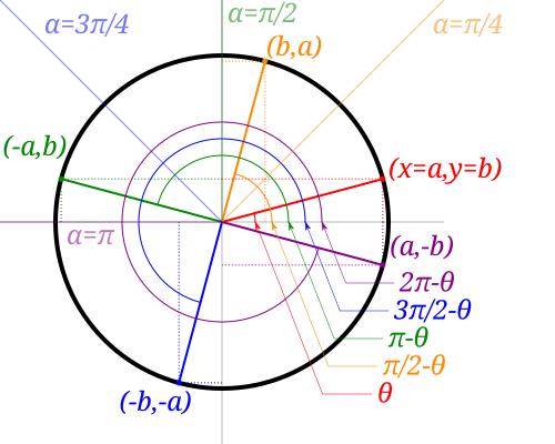
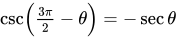
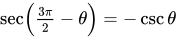
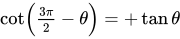
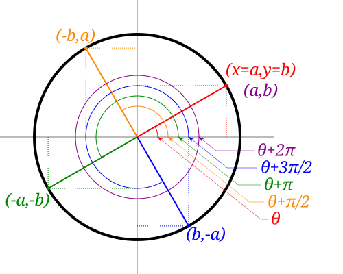
จากการพิจารณาวงกลมหนึ่งหน่วย เราสามารถกำหนดคุณสมบัติต่อไปนี้ของฟังก์ชันตรีโกโนเมตริกได้
ป้าย เครื่องหมายของฟังก์ชันตรีโกณมิติขึ้นอยู่กับควอดแรนต์ของมุม ถ้าและsgn คือฟังก์ชันเครื่องหมาย − π < θ ≤ π {\displaystyle {-\pi }<\theta \leq \pi }
sgn ( sin θ ) = sgn ( csc θ ) = { + 1 if 0 < θ < π − 1 if − π < θ < 0 0 if θ ∈ { 0 , π } sgn ( cos θ ) = sgn ( sec θ ) = { + 1 if − π 2 < θ < π 2 − 1 if − π < θ < − π 2 or π 2 < θ < π 0 if θ ∈ { − π 2 , π 2 } sgn ( tan θ ) = sgn ( cot θ ) = { + 1 if − π < θ < − π 2 or 0 < θ < π 2 − 1 if − π 2 < θ < 0 or π 2 < θ < π 0 if θ ∈ { − π 2 , 0 , π 2 , π } {\displaystyle {\begin{aligned}\operatorname {sgn}(\sin \theta )=\operatorname {sgn}(\csc \theta )&={\begin{cases}+1&{\text{if}}\ \ 0<\theta <\pi \\-1&{\text{if}}\ \ {-\pi }<\theta <0\\0&{\text{if}}\ \ \theta \in \{0,\pi \}\end{cases}}\\[5mu]\operatorname {sgn}(\cos \theta )=\operatorname {sgn}(\sec \theta )&={\begin{cases}+1&{\text{if}}\ \ {-{\tfrac {\pi }{2}}}<\theta <{\tfrac {\pi }{2}}\\-1&{\text{if}}\ \ {-\pi }<\theta <-{\tfrac {\pi }{2}}\ \ {\text{or}}\ \ {\tfrac {\pi }{2}}<\theta <\pi \\0&{\text{if}}\ \ \theta \in {\bigl \{}{-{\tfrac {\pi }{2}}},{\tfrac {\pi }{2}}{\bigr \}}\end{cases}}\\[5mu]\operatorname {sgn}(\tan \theta )=\operatorname {sgn}(\cot \theta )&={\begin{cases}+1&{\text{if}}\ \ {-\pi }<\theta <-{\tfrac {\pi }{2}}\ \ {\text{or}}\ \ 0<\theta <{\tfrac {\pi }{2}}\\-1&{\text{if}}\ \ {-{\tfrac {\pi }{2}}}<\theta <0\ \ {\text{or}}\ \ {\tfrac {\pi }{2}}<\theta <\pi \\0&{\text{if}}\ \ \theta \in {\bigl \{}{-{\tfrac {\pi }{2}}},0,{\tfrac {\pi }{2}},\pi {\bigr \}}\end{cases}}\end{aligned}}}
ฟังก์ชันตรีโกณมิติเป็นฟังก์ชันคาบที่มีคาบร่วมกันดังนั้นสำหรับค่าθ ที่อยู่นอกช่วง ฟังก์ชันจะมีค่าซ้ำกัน (ดูหัวข้อ§ การเลื่อนและคาบ ด้านบน) เครื่องหมายของไซนูซอยด์หรือโคไซนูซอยด์สามารถใช้กำหนดคลื่นสี่เหลี่ยม มาตรฐาน ได้ ตัวอย่างเช่น ฟังก์ชันและจะมีค่า±1 และสอดคล้องกับคลื่นสี่เหลี่ยมที่มีการเลื่อนเฟสเท่ากับ 2 π , {\displaystyle 2\pi ,} ( − π , π ] , {\displaystyle ({-\pi },\pi ],} sgn ( sin x ) {\displaystyle \operatorname {sgn}(\sin x)} sgn ( cos x ) {\displaystyle \operatorname {sgn}(\cos x)} π / 2
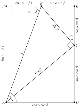
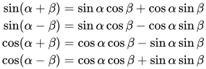
เอกลักษณ์ผลรวมและผลต่างของมุม การสร้างทางเรขาคณิตเพื่อหาเอกลักษณ์ตรีโกณมิติของผลรวมมุม แผนภาพแสดงเอกลักษณ์ความแตกต่างของมุมสำหรับและsin ( α − β ) {\displaystyle \sin(\alpha -\beta )} cos ( α − β ) {\displaystyle \cos(\alpha -\beta )} สิ่งเหล่านี้เรียกอีกอย่างว่า ทฤษฎีบท (หรือสูตร ) การบวกและการลบมุม sin ( α + β ) = sin α cos β + cos α sin β sin ( α − β ) = sin α cos β − cos α sin β cos ( α + β ) = cos α cos β − sin α sin β cos ( α − β ) = cos α cos β + sin α sin β {\displaystyle {\begin{aligned}\sin(\alpha +\beta )&=\sin \alpha \cos \beta +\cos \alpha \sin \beta \\\sin(\alpha -\beta )&=\sin \alpha \cos \beta -\cos \alpha \sin \beta \\\cos(\alpha +\beta )&=\cos \alpha \cos \beta -\sin \alpha \sin \beta \\\cos(\alpha -\beta )&=\cos \alpha \cos \beta +\sin \alpha \sin \beta \end{aligned}}}
เอกลักษณ์ผลต่างมุมสำหรับและสามารถหาได้จากเวอร์ชันผลรวมมุม (และในทางกลับกัน) โดยการแทนที่และโดยใช้ข้อเท็จจริงที่ว่าและนอกจากนี้ยังสามารถหาได้โดยใช้รูปภาพที่ดัดแปลงเล็กน้อยสำหรับเอกลักษณ์ผลรวมมุม ซึ่งแสดงไว้ในที่นี้ และยังสามารถมองได้ว่าเป็นการแสดงผลคูณจุด และผลคูณไขว้ ของเวกเตอร์สองตัวในรูปของโคไซน์และไซน์ของมุมระหว่างเวกเตอร์ ทั้งสองsin ( α − β ) {\displaystyle \sin(\alpha -\beta )} cos ( α − β ) {\displaystyle \cos(\alpha -\beta )} − β {\displaystyle -\beta } β {\displaystyle \beta } sin ( − β ) = − sin ( β ) {\displaystyle \sin(-\beta )=-\sin(\beta )} cos ( − β ) = cos ( β ) {\displaystyle \cos(-\beta )=\cos(\beta )}
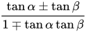
เอกลักษณ์เหล่านี้สรุปไว้ในสองแถวแรกของตารางต่อไปนี้ ซึ่งรวมถึงเอกลักษณ์ผลบวกและผลต่างสำหรับฟังก์ชันตรีโกโนเมตริกอื่นๆ ด้วย
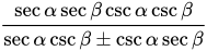
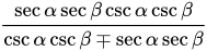
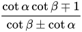
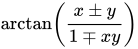
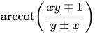
ไซน์ sin ( α ± β ) {\displaystyle \sin(\alpha \pm \beta )} = {\displaystyle =} sin α cos β ± cos α sin β {\displaystyle \sin \alpha \cos \beta \pm \cos \alpha \sin \beta } [ 5 ] [ 6 ] โคไซน์ cos ( α ± β ) {\displaystyle \cos(\alpha \pm \beta )} = {\displaystyle =} cos α cos β ∓ sin α sin β {\displaystyle \cos \alpha \cos \beta \mp \sin \alpha \sin \beta } [ 6 ] [ 7 ] แทนเจนต์ tan ( α ± β ) {\displaystyle \tan(\alpha \pm \beta )} = {\displaystyle =} tan α ± tan β 1 ∓ tan α tan β {\displaystyle {\frac {\tan \alpha \pm \tan \beta }{1\mp \tan \alpha \tan \beta }}} [ 6 ] [ 8 ] โคเซแคนต์ csc ( α ± β ) {\displaystyle \csc(\alpha \pm \beta )} = {\displaystyle =} sec α sec β csc α csc β sec α csc β ± csc α sec β {\displaystyle {\frac {\sec \alpha \sec \beta \csc \alpha \csc \beta }{\sec \alpha \csc \beta \pm \csc \alpha \sec \beta }}} [ 9 ] เซแคนท์ sec ( α ± β ) {\displaystyle \sec(\alpha \pm \beta )} = {\displaystyle =} sec α sec β csc α csc β csc α csc β ∓ sec α sec β {\displaystyle {\frac {\sec \alpha \sec \beta \csc \alpha \csc \beta }{\csc \alpha \csc \beta \mp \sec \alpha \sec \beta }}} [ 9 ] โคแทนเจนต์ cot ( α ± β ) {\displaystyle \cot(\alpha \pm \beta )} = {\displaystyle =} cot α cot β ∓ 1 cot β ± cot α {\displaystyle {\frac {\cot \alpha \cot \beta \mp 1}{\cot \beta \pm \cot \alpha }}} [ 6 ] [ 10 ] อาร์คซีน arcsin x ± arcsin y {\displaystyle \arcsin x\pm \arcsin y} = {\displaystyle =} arcsin ( x 1 − y 2 ± y 1 − x 2 y ) {\displaystyle \arcsin \left(x{\sqrt {1-y^{2}}}\pm y{\sqrt {1-x^{2}{\vphantom {y}}}}\right)} [ 11 ] อาร์คโคซีน arccos x ± arccos y {\displaystyle \arccos x\pm \arccos y} = {\displaystyle =} arccos ( x y ∓ ( 1 − x 2 ) ( 1 − y 2 ) ) {\displaystyle \arccos \left(xy\mp {\sqrt {\left(1-x^{2}\right)\left(1-y^{2}\right)}}\right)} [ 12 ] อาร์คแทงเจนต์ arctan x ± arctan y {\displaystyle \arctan x\pm \arctan y} = {\displaystyle =} arctan ( x ± y 1 ∓ x y ) {\displaystyle \arctan \left({\frac {x\pm y}{1\mp xy}}\right)} [ 13 ] อาร์คโคแทนเจนต์ arccot x ± arccot y {\displaystyle \operatorname {arccot} x\pm \operatorname {arccot} y} = {\displaystyle =} arccot ( x y ∓ 1 y ± x ) {\displaystyle \operatorname {arccot} \left({\frac {xy\mp 1}{y\pm x}}\right)}
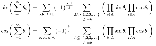
ค่าไซน์และโคไซน์ของผลรวมของมุมจำนวนอนันต์ เมื่ออนุกรมลู่เข้าอย่างสมบูรณ์ แล้ว∑ i = 1 ∞ θ i {\textstyle \sum _{i=1}^{\infty }\theta _{i}}
sin ( ∑ i = 1 ∞ θ i ) = ∑ odd k ≥ 1 ( − 1 ) k − 1 2 ∑ A ⊆ { 1 , 2 , 3 , … } | A | = k ( ∏ i ∈ A sin θ i ∏ i ∉ A cos θ i ) cos ( ∑ i = 1 ∞ θ i ) = ∑ even k ≥ 0 ( − 1 ) k 2 ∑ A ⊆ { 1 , 2 , 3 , … } | A | = k ( ∏ i ∈ A sin θ i ∏ i ∉ A cos θ i ) . {\displaystyle {\begin{aligned}{\sin }{\biggl (}\sum _{i=1}^{\infty }\theta _{i}{\biggl )}&=\sum _{{\text{odd}}\ k\geq 1}(-1)^{\frac {k-1}{2}}\!\!\sum _{\begin{smallmatrix}A\subseteq \{\,1,2,3,\dots \,\}\\\left|A\right|=k\end{smallmatrix}}{\biggl (}\prod _{i\in A}\sin \theta _{i}\prod _{i\not \in A}\cos \theta _{i}{\biggr )}\\{\cos }{\biggl (}\sum _{i=1}^{\infty }\theta _{i}{\biggr )}&=\sum _{{\text{even}}\ k\geq 0}(-1)^{\frac {k}{2}}\,\sum _{\begin{smallmatrix}A\subseteq \{\,1,2,3,\dots \,\}\\\left|A\right|=k\end{smallmatrix}}{\biggl (}\prod _{i\in A}\sin \theta _{i}\prod _{i\not \in A}\cos \theta _{i}{\biggr )}.\end{aligned}}}
เนื่องจากอนุกรมลู่เข้าอย่างสมบูรณ์ จึงจำเป็นต้องเป็นเช่นนั้นและ โดยเฉพาะอย่างยิ่ง ในเอกลักษณ์ทั้งสองนี้ ความไม่สมมาตรปรากฏขึ้นซึ่งไม่พบในกรณีของผลรวมของมุมที่มีจำนวนจำกัด: ในแต่ละผลคูณ จะมีตัวประกอบไซน์เพียงจำนวนจำกัด แต่มี ตัวประกอบโคไซน์จำนวน จำกัด พจน์ที่มีตัวประกอบไซน์จำนวนอนันต์จะต้องเท่ากับศูนย์∑ i = 1 ∞ θ i {\textstyle \sum _{i=1}^{\infty }\theta _{i}} lim i → ∞ θ i = 0 , {\textstyle \lim _{i\to \infty }\theta _{i}=0,} lim i → ∞ sin θ i = 0 , {\textstyle \lim _{i\to \infty }\sin \theta _{i}=0,} lim i → ∞ cos θ i = 1. {\textstyle \lim _{i\to \infty }\cos \theta _{i}=1.}
เมื่อมีเพียงจำนวนจำกัดของมุมที่ไม่เป็นศูนย์ ก็จะมีเพียงจำนวนจำกัดของพจน์ทางด้านขวาที่ไม่เป็นศูนย์เช่นกัน เพราะตัวประกอบไซน์ส่วนใหญ่จะเป็นศูนย์ ยกเว้นเพียงจำนวนจำกัดเท่านั้น ยิ่งไปกว่านั้น ในแต่ละพจน์ ตัวประกอบโคไซน์ส่วนใหญ่จะเป็นหนึ่ง ยกเว้นเพียงจำนวนจำกัดเท่านั้นθ i {\displaystyle \theta _{i}}
เส้นแทนเจนต์และโคแทนเจนต์ของผลรวม ให้(สำหรับ) เป็นพหุนามสมมาตรพื้นฐาน ดีกรีk ในตัวแปร สำหรับนั่นคือe k {\displaystyle e_{k}} k = 0 , 1 , 2 , 3 , … {\displaystyle k=0,1,2,3,\ldots } x i = tan θ i {\displaystyle x_{i}=\tan \theta _{i}} i = 0 , 1 , 2 , 3 , … , {\displaystyle i=0,1,2,3,\ldots ,}
e 0 = 1 e 1 = ∑ i x i = ∑ i tan θ i e 2 = ∑ i < j x i x j = ∑ i < j tan θ i tan θ j e 3 = ∑ i < j < k x i x j x k = ∑ i < j < k tan θ i tan θ j tan θ k ⋮ ⋮ {\displaystyle {\begin{aligned}e_{0}&=1\\[6pt]e_{1}&=\sum _{i}x_{i}&&=\sum _{i}\tan \theta _{i}\\[6pt]e_{2}&=\sum _{i<j}x_{i}x_{j}&&=\sum _{i<j}\tan \theta _{i}\tan \theta _{j}\\[6pt]e_{3}&=\sum _{i<j<k}x_{i}x_{j}x_{k}&&=\sum _{i<j<k}\tan \theta _{i}\tan \theta _{j}\tan \theta _{k}\\&\ \ \vdots &&\ \ \vdots \end{aligned}}}
แล้ว
tan ( ∑ i θ i ) = e 1 − e 3 + e 5 − ⋯ e 0 − e 2 + e 4 − ⋯ . {\displaystyle \tan {\Bigl (}\sum _{i}\theta _{i}{\Bigr )}={\frac {e_{1}-e_{3}+e_{5}-\cdots }{e_{0}-e_{2}+e_{4}-\cdots }}.} tan ( ∑ i θ i ) = sin ( ∑ i θ i ) / ∏ i cos θ i cos ( ∑ i θ i ) / ∏ i cos θ i = ∑ odd k ≥ 1 ( − 1 ) k − 1 2 ∑ A ⊆ { 1 , 2 , 3 , … } | A | = k ∏ i ∈ A tan θ i ∑ even k ≥ 0 ( − 1 ) k 2 ∑ A ⊆ { 1 , 2 , 3 , … } | A | = k ∏ i ∈ A tan θ i = e 1 − e 3 + e 5 − ⋯ e 0 − e 2 + e 4 − ⋯ cot ( ∑ i θ i ) = e 0 − e 2 + e 4 − ⋯ e 1 − e 3 + e 5 − ⋯ {\displaystyle {\begin{aligned}\tan {\Bigl (}\sum _{i}\theta _{i}{\Bigr )}&={\frac {{\sin }{\bigl (}\sum _{i}\theta _{i}{\bigr )}/\prod _{i}\cos \theta _{i}}{{\cos }{\bigl (}\sum _{i}\theta _{i}{\bigr )}/\prod _{i}\cos \theta _{i}}}\\[10pt]&={\frac {\displaystyle \sum _{{\text{odd}}\ k\geq 1}(-1)^{\frac {k-1}{2}}\sum _{\begin{smallmatrix}A\subseteq \{1,2,3,\dots \}\\\left|A\right|=k\end{smallmatrix}}\prod _{i\in A}\tan \theta _{i}}{\displaystyle \sum _{{\text{even}}\ k\geq 0}~(-1)^{\frac {k}{2}}~~\sum _{\begin{smallmatrix}A\subseteq \{1,2,3,\dots \}\\\left|A\right|=k\end{smallmatrix}}\prod _{i\in A}\tan \theta _{i}}}={\frac {e_{1}-e_{3}+e_{5}-\cdots }{e_{0}-e_{2}+e_{4}-\cdots }}\\[10pt]\cot {\Bigl (}\sum _{i}\theta _{i}{\Bigr )}&={\frac {e_{0}-e_{2}+e_{4}-\cdots }{e_{1}-e_{3}+e_{5}-\cdots }}\end{aligned}}}
จำนวนพจน์ทางด้านขวาขึ้นอยู่กับจำนวนพจน์ทางด้านซ้าย
ตัวอย่างเช่น: tan ( θ 1 + θ 2 ) = e 1 e 0 − e 2 = x 1 + x 2 1 − x 1 x 2 = tan θ 1 + tan θ 2 1 − tan θ 1 tan θ 2 , tan ( θ 1 + θ 2 + θ 3 ) = e 1 − e 3 e 0 − e 2 = ( x 1 + x 2 + x 3 ) − ( x 1 x 2 x 3 ) 1 − ( x 1 x 2 + x 1 x 3 + x 2 x 3 ) , tan ( θ 1 + θ 2 + θ 3 + θ 4 ) = e 1 − e 3 e 0 − e 2 + e 4 = ( x 1 + x 2 + x 3 + x 4 ) − ( x 1 x 2 x 3 + x 1 x 2 x 4 + x 1 x 3 x 4 + x 2 x 3 x 4 ) 1 − ( x 1 x 2 + x 1 x 3 + x 1 x 4 + x 2 x 3 + x 2 x 4 + x 3 x 4 ) + ( x 1 x 2 x 3 x 4 ) , {\displaystyle {\begin{aligned}\tan(\theta _{1}+\theta _{2})&={\frac {e_{1}}{e_{0}-e_{2}}}={\frac {x_{1}+x_{2}}{1\ -\ x_{1}x_{2}}}={\frac {\tan \theta _{1}+\tan \theta _{2}}{1\ -\ \tan \theta _{1}\tan \theta _{2}}},\\[8pt]\tan(\theta _{1}+\theta _{2}+\theta _{3})&={\frac {e_{1}-e_{3}}{e_{0}-e_{2}}}={\frac {(x_{1}+x_{2}+x_{3})\ -\ (x_{1}x_{2}x_{3})}{1\ -\ (x_{1}x_{2}+x_{1}x_{3}+x_{2}x_{3})}},\\[8pt]\tan(\theta _{1}+\theta _{2}+\theta _{3}+\theta _{4})&={\frac {e_{1}-e_{3}}{e_{0}-e_{2}+e_{4}}}\\[8pt]&={\frac {(x_{1}+x_{2}+x_{3}+x_{4})\ -\ (x_{1}x_{2}x_{3}+x_{1}x_{2}x_{4}+x_{1}x_{3}x_{4}+x_{2}x_{3}x_{4})}{1\ -\ (x_{1}x_{2}+x_{1}x_{3}+x_{1}x_{4}+x_{2}x_{3}+x_{2}x_{4}+x_{3}x_{4})\ +\ (x_{1}x_{2}x_{3}x_{4})}},\end{aligned}}}
และอื่นๆ กรณีที่มีพจน์จำนวนจำกัดเท่านั้นสามารถพิสูจน์ได้ด้วย การเหนี่ยว นำทางคณิตศาสตร์ [ 14 ] [ 15 ]
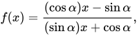
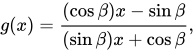
สมมติว่าและและa , b , c , d , p , q ∈ R {\textstyle a,b,c,d,p,q\in \mathbb {R} } i = − 1 {\textstyle i={\sqrt {-1}}}
a i + b c i + d = p i + q {\displaystyle {\frac {ai+b}{ci+d}}=pi+q} และให้เป็นจำนวนใดๆ ซึ่ง สมมติว่าดังนั้นเศษส่วนข้างต้นจึงไม่สามารถเป็น φ {\textstyle \varphi } tan φ = c d . {\textstyle \tan \varphi ={\tfrac {c}{d}}.} a c ≠ b d {\textstyle {\tfrac {a}{c}}\neq {\tfrac {b}{d}}} 0 / 0 . [ 16 ] θ ∈ R {\textstyle \theta \in \mathbb {R} }
a tan θ + b c tan θ + d = p tan ( θ − φ ) + q . {\displaystyle {\frac {a\tan \theta +b}{c\tan \theta +d}}=p\tan(\theta -\varphi )+q.} (ในกรณีที่ตัวส่วนของเศษส่วนนี้เป็น 0 เราจะกำหนดค่าของเศษส่วนเป็นโดยที่สัญลักษณ์ไม่ได้หมายถึงหรือแต่หมายถึงค่าที่เข้าใกล้โดยการเคลื่อนที่ไปในทิศทางบวกหรือลบ ทำให้การเติมเต็มเส้นตรงนั้นในทางโทโพโลยีเป็นวงกลม)∞ {\textstyle \infty } ∞ {\textstyle \infty } + ∞ {\textstyle +\infty } − ∞ {\textstyle -\infty } ∞ {\textstyle \infty } R ∪ { ∞ } {\textstyle \mathbb {R} \cup \{\,\infty \,\}}
จากเอกลักษณ์นี้สามารถแสดงให้เห็นได้อย่างรวดเร็วว่าตระกูลของ ตัวแปรสุ่ม ที่มีการแจกแจงแบบโคชี ทั้งหมด นั้นปิดภายใต้การแปลงเศษส่วนเชิงเส้น ซึ่งเป็นผลลัพธ์ที่ทราบกันมาตั้งแต่ปี พ.ศ. 2519 [ 17 ]
เส้นตัดและเส้นร่วมตัดของผลรวม sec ( ∑ i θ i ) = ∏ i sec θ i e 0 − e 2 + e 4 − ⋯ csc ( ∑ i θ i ) = ∏ i sec θ i e 1 − e 3 + e 5 − ⋯ {\displaystyle {\begin{aligned}{\sec }{\Bigl (}\sum _{i}\theta _{i}{\Bigr )}&={\frac {\prod _{i}\sec \theta _{i}}{e_{0}-e_{2}+e_{4}-\cdots }}\\[8pt]{\csc }{\Bigl (}\sum _{i}\theta _{i}{\Bigr )}&={\frac {\prod _{i}\sec \theta _{i}}{e_{1}-e_{3}+e_{5}-\cdots }}\end{aligned}}}
โดยที่พหุนามสมมาตรพื้นฐานดีกรี k ในตัวแปรn ตัวและจำนวนพจน์ในตัวส่วนและจำนวนตัวประกอบในผลคูณในตัวเศษขึ้นอยู่กับจำนวนพจน์ในผลรวมทางด้านซ้าย[ 18 ] e k {\displaystyle e_{k}} x i = tan θ i , {\displaystyle x_{i}=\tan \theta _{i},} i = 1 , … , n , {\displaystyle i=1,\ldots ,n,}
ตัวอย่างเช่น,
sec ( α + β + γ ) = sec α sec β sec γ 1 − tan α tan β − tan α tan γ − tan β tan γ csc ( α + β + γ ) = sec α sec β sec γ tan α + tan β + tan γ − tan α tan β tan γ . {\displaystyle {\begin{aligned}\sec(\alpha +\beta +\gamma )&={\frac {\sec \alpha \sec \beta \sec \gamma }{1-\tan \alpha \tan \beta -\tan \alpha \tan \gamma -\tan \beta \tan \gamma }}\\[8pt]\csc(\alpha +\beta +\gamma )&={\frac {\sec \alpha \sec \beta \sec \gamma }{\tan \alpha +\tan \beta +\tan \gamma -\tan \alpha \tan \beta \tan \gamma }}.\end{aligned}}}
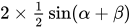
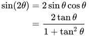
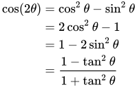
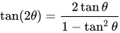
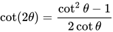
การสาธิตเชิงภาพของสูตรมุมสองเท่าสำหรับค่าไซน์ สำหรับสามเหลี่ยมหน้าจั่วข้างต้นที่มีด้านยาวหนึ่งหน่วยและมุม 2θ พื้นที่ 1 / 2 ( sinθ cosθ เมื่อวางตะแคง พื้นที่เดียวกันคือ 1 / 2 บาป θ ดังนั้นบาปθ = 2ซินθ cosθ .
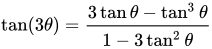
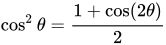
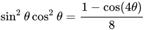
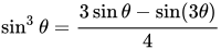
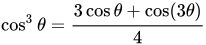
สูตรสำหรับมุมสามเท่า[ 20 ]
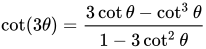
sin ( 3 θ ) = 3 sin θ − 4 sin 3 θ = 4 sin θ sin ( π 3 − θ ) sin ( π 3 + θ ) cos ( 3 θ ) = 4 cos 3 θ − 3 cos θ = 4 cos θ cos ( π 3 − θ ) cos ( π 3 + θ ) tan ( 3 θ ) = 3 tan θ − tan 3 θ 1 − 3 tan 2 θ = tan θ tan ( π 3 − θ ) tan ( π 3 + θ ) cot ( 3 θ ) = 3 cot θ − cot 3 θ 1 − 3 cot 2 θ sec ( 3 θ ) = sec 3 θ 4 − 3 sec 2 θ csc ( 3 θ ) = csc 3 θ 3 csc 2 θ − 4 {\displaystyle {\begin{aligned}\sin(3\theta )&=3\sin \theta -4\sin ^{3}\theta &&=4\sin \theta \sin \left({\tfrac {\pi }{3}}-\theta \right)\sin \left({\tfrac {\pi }{3}}+\theta \right)\\\cos(3\theta )&=4\cos ^{3}\theta -3\cos \theta &&=4\cos \theta \cos \left({\tfrac {\pi }{3}}-\theta \right)\cos \left({\tfrac {\pi }{3}}+\theta \right)\\\tan(3\theta )&={\frac {3\tan \theta -\tan ^{3}\theta }{1-3\tan ^{2}\theta }}&&=\tan \theta \tan \left({\tfrac {\pi }{3}}-\theta \right)\tan \left({\tfrac {\pi }{3}}+\theta \right)\\\cot(3\theta )&={\frac {3\cot \theta -\cot ^{3}\theta }{1-3\cot ^{2}\theta }}\\\sec(3\theta )&={\frac {\sec ^{3}\theta }{4-3\sec ^{2}\theta }}\\\csc(3\theta )&={\frac {\csc ^{3}\theta }{3\csc ^{2}\theta -4}}\\\end{aligned}}}
สูตรสำหรับมุมหลายมุม[ 22 ]
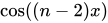
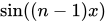
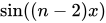
sin ( n θ ) = ∑ k ∈ O + n ( − 1 ) k − 1 2 ( n k ) cos n − k θ sin k θ = sin θ ∑ i = 0 n + 1 2 ∑ j = 0 i ( − 1 ) i − j ( n 2 i + 1 ) ( i j ) cos n − 2 ( i − j ) − 1 θ = sin ( θ ) ∑ k = 0 ⌊ n − 1 2 ⌋ ( − 1 ) k ( 2 cos ( θ ) ) n − 2 k − 1 ( n − k − 1 k ) = 2 ( n − 1 ) ∏ k = 0 n − 1 sin ( k π n + θ ) cos ( n θ ) = ∑ k ∈ E 0 + n ( − 1 ) k 2 ( n k ) cos n − k θ sin k θ = ∑ i = 0 n 2 ∑ j = 0 i ( − 1 ) i − j ( n 2 i ) ( i j ) cos n − 2 ( i − j ) θ = ∑ k = 0 ⌊ n 2 ⌋ ( − 1 ) k ( 2 cos ( θ ) ) n − 2 k ( n − k k ) n 2 n − 2 k cos ( ( 2 n + 1 ) θ ) = ( − 1 ) n 2 2 n ∏ k = 0 2 n cos ( k π 2 n + 1 − θ ) cos ( 2 n θ ) = ( − 1 ) n 2 2 n − 1 ∏ k = 0 2 n − 1 cos ( ( 1 + 2 k ) π 4 n − θ ) tan ( n θ ) = ∑ k ∈ O + n ( − 1 ) k − 1 2 ( n k ) tan k θ ∑ k ∈ E 0 + n ( − 1 ) k 2 ( n k ) tan k θ O + = Positive odd integers E 0 + = Non-negative even integers {\displaystyle {\begin{aligned}\sin(n\theta )&=\sum _{k\in \mathbb {O} ^{+}}^{n}(-1)^{\frac {k-1}{2}}{n \choose k}\cos ^{n-k}\theta \sin ^{k}\theta =\sin \theta \sum _{i=0}^{\frac {n+1}{2}}\sum _{j=0}^{i}(-1)^{i-j}{n \choose 2i+1}{i \choose j}\cos ^{n-2(i-j)-1}\theta \\&=\sin(\theta )\sum _{k=0}^{\left\lfloor {\frac {n-1}{2}}\right\rfloor }(-1)^{k}{\bigl (}2\cos(\theta ){\bigr )}^{n-2k-1}{n-k-1 \choose k}\\&=2^{(n-1)}\prod _{k=0}^{n-1}\sin \left({\frac {k\pi }{n}}+\theta \right)\\\cos(n\theta )&=\sum _{k\in \mathbb {E} _{0}^{+}}^{n}(-1)^{\frac {k}{2}}{n \choose k}\cos ^{n-k}\theta \sin ^{k}\theta =\sum _{i=0}^{\frac {n}{2}}\sum _{j=0}^{i}(-1)^{i-j}{n \choose 2i}{i \choose j}\cos ^{n-2(i-j)}\theta \\&=\sum _{k=0}^{\left\lfloor {\frac {n}{2}}\right\rfloor }(-1)^{k}{(2\cos(\theta ))}^{n-2k}{n-k \choose k}{\frac {n}{2n-2k}}\\\cos {\bigl (}(2n+1)\theta {\bigr )}&=(-1)^{n}2^{2n}\prod _{k=0}^{2n}\cos \left({\frac {k\pi }{2n+1}}-\theta \right)\\\cos(2n\theta )&=(-1)^{n}2^{2n-1}\prod _{k=0}^{2n-1}\cos \left({\frac {(1+2k)\pi }{4n}}-\theta \right)\\\tan(n\theta )&={\frac {\displaystyle \sum _{k\in \mathbb {O} ^{+}}^{n}(-1)^{\frac {k-1}{2}}{n \choose k}\tan ^{k}\theta }{\displaystyle \sum _{k\in \mathbb {E} _{0}^{+}}^{n}(-1)^{\frac {k}{2}}{n \choose k}\tan ^{k}\theta }}\\\mathbb {O} ^{+}&={\text{Positive odd integers}}\\\mathbb {E} _{0}^{+}&={\text{Non-negative even integers}}\\\end{aligned}}}
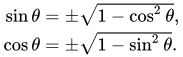
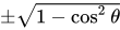
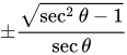
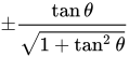
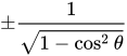
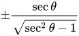
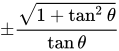
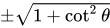
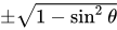
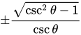
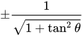
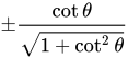
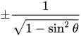
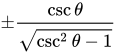
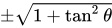
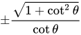
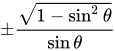
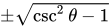
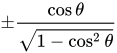
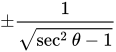
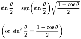
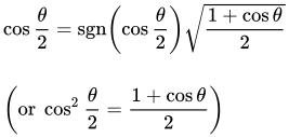
sin θ 2 = sgn ( sin θ 2 ) 1 − cos θ 2 cos θ 2 = sgn ( cos θ 2 ) 1 + cos θ 2 tan θ 2 = 1 − cos θ sin θ = sin θ 1 + cos θ = csc θ − cot θ = tan θ 1 + sec θ = sgn ( sin θ ) 1 − cos θ 1 + cos θ = − 1 + sgn ( cos θ ) 1 + tan 2 θ tan θ cot θ 2 = 1 + cos θ sin θ = sin θ 1 − cos θ = csc θ + cot θ = sgn ( sin θ ) 1 + cos θ 1 − cos θ sec θ 2 = sgn ( cos θ 2 ) 2 1 + cos θ csc θ 2 = sgn ( sin θ 2 ) 2 1 − cos θ {\displaystyle {\begin{aligned}\sin {\frac {\theta }{2}}&=\operatorname {sgn} \left(\sin {\frac {\theta }{2}}\right){\sqrt {\frac {1-\cos \theta }{2}}}\\[3pt]\cos {\frac {\theta }{2}}&=\operatorname {sgn} \left(\cos {\frac {\theta }{2}}\right){\sqrt {\frac {1+\cos \theta }{2}}}\\[3pt]\tan {\frac {\theta }{2}}&={\frac {1-\cos \theta }{\sin \theta }}={\frac {\sin \theta }{1+\cos \theta }}=\csc \theta -\cot \theta ={\frac {\tan \theta }{1+\sec {\theta }}}\\[6mu]&=\operatorname {sgn}(\sin \theta ){\sqrt {\frac {1-\cos \theta }{1+\cos \theta }}}={\frac {-1+\operatorname {sgn}(\cos \theta ){\sqrt {1+\tan ^{2}\theta }}}{\tan \theta }}\\[3pt]\cot {\frac {\theta }{2}}&={\frac {1+\cos \theta }{\sin \theta }}={\frac {\sin \theta }{1-\cos \theta }}=\csc \theta +\cot \theta =\operatorname {sgn}(\sin \theta ){\sqrt {\frac {1+\cos \theta }{1-\cos \theta }}}\\\sec {\frac {\theta }{2}}&=\operatorname {sgn} \left(\cos {\frac {\theta }{2}}\right){\sqrt {\frac {2}{1+\cos \theta }}}\\\csc {\frac {\theta }{2}}&=\operatorname {sgn} \left(\sin {\frac {\theta }{2}}\right){\sqrt {\frac {2}{1-\cos \theta }}}\\\end{aligned}}} [ 25 ] [ 26 ]
อีกด้วย tan η ± θ 2 = sin η ± sin θ cos η + cos θ tan ( θ 2 + π 4 ) = sec θ + tan θ 1 − sin θ 1 + sin θ = | 1 − tan θ 2 | | 1 + tan θ 2 | {\displaystyle {\begin{aligned}\tan {\frac {\eta \pm \theta }{2}}&={\frac {\sin \eta \pm \sin \theta }{\cos \eta +\cos \theta }}\\[3pt]\tan \left({\frac {\theta }{2}}+{\frac {\pi }{4}}\right)&=\sec \theta +\tan \theta \\[3pt]{\sqrt {\frac {1-\sin \theta }{1+\sin \theta }}}&={\frac {\left|1-\tan {\frac {\theta }{2}}\right|}{\left|1+\tan {\frac {\theta }{2}}\right|}}\end{aligned}}}
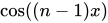
เอกลักษณ์ผลคูณเป็นผลรวมและเอกลักษณ์ผลรวมเป็นผลคูณ การพิสูจน์เอกลักษณ์โคไซน์ผลรวมและผลต่างสำหรับการคำนวณโปรสตาเฟอรีซิสโดยใช้สามเหลี่ยมหน้าจั่ว เอกลักษณ์ผลคูณเป็นผลรวม[ 30 ] โปรสตาเฟอรีซิส สามารถพิสูจน์ได้โดยการขยายด้านขวาโดยใช้ทฤษฎีบทการบวกมุม ในอดีต สี่ข้อแรกเหล่านี้เรียกว่าสูตรของเวอร์เนอร์ ตามชื่อ ของ โยฮันเนส เวอร์เนอร์ ผู้ใช้สูตรเหล่านี้ในการคำนวณทางดาราศาสตร์[ 31 ] การปรับแอมพลิจูด สำหรับการประยุกต์ใช้สูตรผลคูณเป็นผลรวม และบีท (อะคูสติก) และตัวตรวจจับเฟส สำหรับการประยุกต์ใช้สูตรผลรวมเป็นผลคูณ
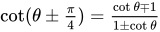
เอกลักษณ์ผลคูณเป็นผลรวม ผลคูณของค่าไซน์หรือโคไซน์สองค่าที่มีมุมต่างกัน สามารถแปลงเป็นผลรวมของฟังก์ชันตรีโกโนเมตริกของผลรวมและผลต่างของมุมเหล่านั้นได้:
cos θ cos φ = 1 2 ( cos ( θ − φ ) + cos ( θ + φ ) ) , sin θ sin φ = 1 2 ( cos ( θ − φ ) − cos ( θ + φ ) ) , sin θ cos φ = 1 2 ( sin ( θ + φ ) + sin ( θ − φ ) ) , cos θ sin φ = 1 2 ( sin ( θ + φ ) − sin ( θ − φ ) ) . {\displaystyle {\begin{aligned}\cos \theta \,\cos \varphi &={\tfrac {1}{2}}{\bigl (}\!\!~\cos(\theta -\varphi )+\cos(\theta +\varphi ){\bigr )},\\[5mu]\sin \theta \,\sin \varphi &={\tfrac {1}{2}}{\bigl (}\!\!~\cos(\theta -\varphi )-\cos(\theta +\varphi ){\bigr )},\\[5mu]\sin \theta \,\cos \varphi &={\tfrac {1}{2}}{\bigl (}\!\!~\sin(\theta +\varphi )+\sin(\theta -\varphi ){\bigr )},\\[5mu]\cos \theta \,\sin \varphi &={\tfrac {1}{2}}{\bigl (}\!\!~\sin(\theta +\varphi )-\sin(\theta -\varphi ){\bigr )}.\end{aligned}}} tan θ tan φ = cos ( θ − φ ) − cos ( θ + φ ) cos ( θ − φ ) + cos ( θ + φ ) , tan θ tan φ = sin ( θ + φ ) + sin ( θ − φ ) sin ( θ + φ ) − sin ( θ − φ ) . {\displaystyle {\begin{aligned}\tan \theta \,\tan \varphi &={\frac {\cos(\theta -\varphi )-\cos(\theta +\varphi )}{\cos(\theta -\varphi )+\cos(\theta +\varphi )}},\\[5mu]{\frac {\tan \theta }{\tan \varphi }}&={\frac {\sin(\theta +\varphi )+\sin(\theta -\varphi )}{\sin(\theta +\varphi )-\sin(\theta -\varphi )}}.\end{aligned}}}
โดยทั่วไปแล้ว สำหรับผลคูณของค่าไซน์หรือโคไซน์จำนวนใดๆ ก็ตาม∏ k = 1 n cos θ k = 1 2 n ∑ e ∈ S cos ( e 1 θ 1 + ⋯ + e n θ n ) where e = ( e 1 , … , e n ) ∈ S = { 1 , − 1 } n , ∏ k = 1 n sin θ k = ( − 1 ) ⌊ n 2 ⌋ 2 n { ∑ e ∈ S cos ( e 1 θ 1 + ⋯ + e n θ n ) ∏ j = 1 n e j if n is even , ∑ e ∈ S sin ( e 1 θ 1 + ⋯ + e n θ n ) ∏ j = 1 n e j if n is odd . {\displaystyle {\begin{aligned}\prod _{k=1}^{n}\cos \theta _{k}&={\frac {1}{2^{n}}}\sum _{e\in S}\cos(e_{1}\theta _{1}+\cdots +e_{n}\theta _{n})\\[5mu]&{\text{where }}e=(e_{1},\ldots ,e_{n})\in S=\{1,-1\}^{n},\\\prod _{k=1}^{n}\sin \theta _{k}&={\frac {(-1)^{\left\lfloor {\frac {n}{2}}\right\rfloor }}{2^{n}}}{\begin{cases}\displaystyle \sum _{e\in S}\cos(e_{1}\theta _{1}+\cdots +e_{n}\theta _{n})\prod _{j=1}^{n}e_{j}\;{\text{if}}\;n\;{\text{is even}},\\\displaystyle \sum _{e\in S}\sin(e_{1}\theta _{1}+\cdots +e_{n}\theta _{n})\prod _{j=1}^{n}e_{j}\;{\text{if}}\;n\;{\text{is odd}}.\end{cases}}\end{aligned}}}
เอกลักษณ์ผลรวมเป็นผลคูณ แผนภาพแสดงความสัมพันธ์ระหว่างผลรวมและผลคูณของฟังก์ชันไซน์และโคไซน์ สามเหลี่ยมมุมฉากสีน้ำเงินมีมุม θ และสามเหลี่ยมมุมฉากสีแดงมีมุมθ ทั้งสองมีด้านตรงข้ามมุมฉากยาว 1 มุมเสริมที่เรียกว่า θ และθ ถูกสร้างขึ้นเพื่อให้θ และ θ = θ และ θ = θ ดังนั้น θ และ θ = θ ซึ่งทำให้สามารถสร้างสามเหลี่ยมที่มีเส้นขอบสีม่วงที่เท่ากันทุกประการสองรูป คือ θ และθ โดยแต่ละรูปมีด้านตรงข้ามมุมฉากและมุม θ ที่ฐาน ผลรวมของความสูงของสามเหลี่ยมสีแดงและสีน้ำเงินคือ θ = 1 และ θ = 2 ซึ่งเท่ากับสองเท่าของความสูงของสามเหลี่ยมสีม่วงรูปหนึ่ง นั่นคือ θ = 1 เมื่อเขียน θ และθ ในสมการนั้นในรูปของ θ และ θ จะได้ความสัมพันธ์ระหว่างผลรวมและ ผลคูณของฟังก์ชันไซน์ คือ θ = 1 ในทำนองเดียวกัน ผลรวมของความกว้างของสามเหลี่ยมสีแดงและสีน้ำเงินจะให้ความสัมพันธ์ที่สอดคล้องกันสำหรับฟังก์ชันโคไซน์θ {\displaystyle \theta } φ {\displaystyle \varphi } p {\displaystyle p} q {\displaystyle q} p = 1 2 ( θ + φ ) {\displaystyle p={\tfrac {1}{2}}(\theta +\varphi )} q = 1 2 ( θ − φ ) {\displaystyle q={\tfrac {1}{2}}(\theta -\varphi )} θ = p + q {\displaystyle \theta =p+q} φ = p − q {\displaystyle \varphi =p-q} A F G {\displaystyle AFG} F C E {\displaystyle FCE} cos q {\displaystyle \cos q} p {\displaystyle p} sin θ + sin φ {\displaystyle \sin \theta +\sin \varphi } 2 sin p cos q {\displaystyle 2\sin p\cos q} p {\displaystyle p} q {\displaystyle q} θ {\displaystyle \theta } φ {\displaystyle \varphi } sin θ + sin φ = 2 sin 1 2 ( θ + φ ) cos 1 2 ( θ − φ ) {\displaystyle \sin \theta +\sin \varphi =2\sin {\tfrac {1}{2}}(\theta +\varphi )\,\cos {\tfrac {1}{2}}(\theta -\varphi )} ผลรวมของไซน์หรือโคไซน์ของมุมสองมุมสามารถแปลงเป็นผลคูณของไซน์หรือโคไซน์ของค่าเฉลี่ยและครึ่งหนึ่งของผลต่างของมุมได้: [ 32 ]
sin θ + sin φ = 2 sin 1 2 ( θ + φ ) cos 1 2 ( θ − φ ) , sin θ − sin φ = 2 cos 1 2 ( θ + φ ) sin 1 2 ( θ − φ ) , cos θ + cos φ = 2 cos 1 2 ( θ + φ ) cos 1 2 ( θ − φ ) , cos θ − cos φ = − 2 sin 1 2 ( θ + φ ) sin 1 2 ( θ − φ ) . {\displaystyle {\begin{aligned}\sin \theta +\sin \varphi &=2\sin {\tfrac {1}{2}}(\theta +\varphi )\,\cos {\tfrac {1}{2}}(\theta -\varphi ),\\[5mu]\sin \theta -\sin \varphi &=2\cos {\tfrac {1}{2}}(\theta +\varphi )\,\sin {\tfrac {1}{2}}(\theta -\varphi ),\\[5mu]\cos \theta +\cos \varphi &=2\cos {\tfrac {1}{2}}(\theta +\varphi )\,\cos {\tfrac {1}{2}}(\theta -\varphi ),\\[5mu]\cos \theta -\cos \varphi &=-2\sin {\tfrac {1}{2}}(\theta +\varphi )\,\sin {\tfrac {1}{2}}(\theta -\varphi ).\end{aligned}}}
ผลรวมของแทนเจนต์ของมุมสองมุมสามารถแปลงเป็นผลหารของไซน์ของมุมหารด้วยผลคูณของโคไซน์ได้: [ 32 ] tan θ ± tan φ = sin ( θ ± φ ) cos θ cos φ . {\displaystyle \tan \theta \pm \tan \varphi ={\frac {\sin(\theta \pm \varphi )}{\cos \theta \,\cos \varphi }}.}
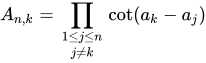
Charles Hermite ได้แสดงเอกลักษณ์ต่อไปนี้[ 33 ] จำนวนเชิงซ้อน ซึ่งไม่มีจำนวนเชิงซ้อนใดที่แตกต่างกันด้วยผลคูณจำนวนเต็มของπ ให้a 1 , … , a n {\displaystyle a_{1},\ldots ,a_{n}}
A n , k = ∏ 1 ≤ j ≤ n j ≠ k cot ( a k − a j ) {\displaystyle A_{n,k}=\prod _{\begin{smallmatrix}1\leq j\leq n\\j\neq k\end{smallmatrix}}\cot(a_{k}-a_{j})}
(โดยเฉพาะอย่างยิ่งการเป็นผลิตภัณฑ์ที่ว่างเปล่า คือ1) จากนั้นA 1 , 1 , {\displaystyle A_{1,1},}
cot ( z − a 1 ) ⋯ cot ( z − a n ) = cos n π 2 + ∑ k = 1 n A n , k cot ( z − a k ) . {\displaystyle \cot(z-a_{1})\cdots \cot(z-a_{n})=\cos {\frac {n\pi }{2}}+\sum _{k=1}^{n}A_{n,k}\cot(z-a_{k}).}
ตัวอย่างที่ไม่ธรรมดาที่ง่ายที่สุดคือกรณีn = 2 :
cot ( z − a 1 ) cot ( z − a 2 ) = − 1 + cot ( a 1 − a 2 ) cot ( z − a 1 ) + cot ( a 2 − a 1 ) cot ( z − a 2 ) . {\displaystyle \cot(z-a_{1})\cot(z-a_{2})=-1+\cot(a_{1}-a_{2})\cot(z-a_{1})+\cot(a_{2}-a_{1})\cot(z-a_{2}).}
ผลคูณจำกัดของฟังก์ชันตรีโกณมิติ สำหรับจำนวนเต็มn , m ที่เป็นจำนวน เฉพาะสัมพัทธ์
∏ k = 1 n ( 2 a + 2 cos ( 2 π k m n + x ) ) = 2 ( T n ( a ) + ( − 1 ) n + m cos ( n x ) ) {\displaystyle \prod _{k=1}^{n}\left(2a+2\cos \left({\frac {2\pi km}{n}}+x\right)\right)=2\left(T_{n}(a)+{(-1)}^{n+m}\cos(nx)\right)}
โดยที่T คือพหุนามเชบิ เชฟ
ความสัมพันธ์ต่อไปนี้ใช้ได้กับฟังก์ชันไซน์
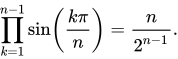
∏ k = 1 n − 1 sin ( k π n ) = n 2 n − 1 . {\displaystyle \prod _{k=1}^{n-1}\sin \left({\frac {k\pi }{n}}\right)={\frac {n}{2^{n-1}}}.}
โดยทั่วไปสำหรับจำนวนเต็มn > 0 [ 34 ]
sin ( n x ) = 2 n − 1 ∏ k = 0 n − 1 sin ( k π n + x ) = 2 n − 1 ∏ k = 1 n sin ( k π n − x ) . {\displaystyle \sin(nx)=2^{n-1}\prod _{k=0}^{n-1}\sin \left({\frac {k\pi }{n}}+x\right)=2^{n-1}\prod _{k=1}^{n}\sin \left({\frac {k\pi }{n}}-x\right).}
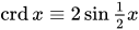
หรือเขียนในแง่ของหน้าที่ของคอร์ด crd x ≡ 2 sin 1 2 x {\textstyle \operatorname {crd} x\equiv 2\sin {\tfrac {1}{2}}x}
crd ( n x ) = ∏ k = 1 n crd ( 2 k π n − x ) . {\displaystyle \operatorname {crd} (nx)=\prod _{k=1}^{n}\operatorname {crd} \left({\frac {2k\pi }{n}}-x\right).}
สิ่งนี้มาจากการแยกตัวประกอบของพหุนาม ออกเป็นตัวประกอบเชิงเส้น (ดูรากที่หนึ่ง ): สำหรับจำนวนเชิงซ้อนz ใดๆ และจำนวนเต็มn > 0z n − 1 {\textstyle z^{n}-1}
z n − 1 = ∏ k = 1 n ( z − exp 2 k i π n ) . {\displaystyle z^{n}-1=\prod _{k=1}^{n}\left(z-\exp {\frac {2ki\pi }{n}}\right).}
การรวมเชิงเส้น ในบางวัตถุประสงค์ เป็นเรื่องสำคัญที่จะต้องทราบว่าการรวมกันเชิงเส้น ของคลื่นไซน์ที่มีคาบหรือความถี่เดียวกัน แต่มีเฟส ต่างกัน ก็ยังคงได้เป็นคลื่นไซน์ที่มีคาบหรือความถี่เดียวกัน แต่มีเฟสต่างกันเช่นกัน สิ่งนี้มีประโยชน์ในการปรับข้อมูล ไซน์ให้ เข้ากับแบบจำลอง เนื่องจากข้อมูลที่วัดหรือสังเกตได้มีความสัมพันธ์เชิงเส้นกับตัวแปร ที่ไม่ทราบค่า a และb ของ ฐาน ส่วนประกอบเฟสตรงกันและเฟสตั้งฉาก ด้านล่าง ส่งผลให้เมท ริกซ์จาโคเบียน ง่ายขึ้นเมื่อเทียบกับเมทริกซ์ของและc {\displaystyle c} φ {\displaystyle \varphi }
ไซน์และโคไซน์ การรวมเชิงเส้นหรือการบวกฮาร์มอนิกของคลื่นไซน์และโคไซน์เทียบเท่ากับคลื่นไซน์เดี่ยวที่มีการเลื่อนเฟสและแอมพลิจูดที่ปรับขนาด[ 35 ] [ 36 ]
a cos x + b sin x = c cos ( x + φ ) {\displaystyle a\cos x+b\sin x=c\cos(x+\varphi )}
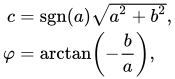
โดยที่และถูกกำหนดไว้ดังนี้:c {\displaystyle c} φ {\displaystyle \varphi }
c = sgn ( a ) a 2 + b 2 , φ = arctan ( − b a ) , {\displaystyle {\begin{aligned}c&=\operatorname {sgn}(a){\sqrt {a^{2}+b^{2}}},\\\varphi &=\arctan \left(-{\frac {b}{a}}\right),\end{aligned}}}
เนื่องจากa ≠ 0. {\displaystyle a\neq 0.}
การเลื่อนเฟสตามอำเภอใจ โดยทั่วไปแล้ว สำหรับการเลื่อนเฟสใดๆ เราจะได้ว่า
a sin ( x + θ a ) + b sin ( x + θ b ) = c sin ( x + φ ) {\displaystyle a\sin(x+\theta _{a})+b\sin(x+\theta _{b})=c\sin(x+\varphi )}
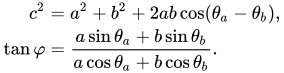
ที่ไหนและตอบสนอง:c {\displaystyle c} φ {\displaystyle \varphi }
c 2 = a 2 + b 2 + 2 a b cos ( θ a − θ b ) , tan φ = a sin θ a + b sin θ b a cos θ a + b cos θ b . {\displaystyle {\begin{aligned}c^{2}&=a^{2}+b^{2}+2ab\cos \left(\theta _{a}-\theta _{b}\right),\\\tan \varphi &={\frac {a\sin \theta _{a}+b\sin \theta _{b}}{a\cos \theta _{a}+b\cos \theta _{b}}}.\end{aligned}}}
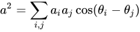
ไซนูซอยด์มากกว่าสองอัน กรณีทั่วไปอ่านว่า[ 36 ]
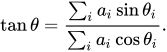
∑ i a i sin ( x + θ i ) = a sin ( x + θ ) , {\displaystyle \sum _{i}a_{i}\sin(x+\theta _{i})=a\sin(x+\theta ),} a 2 = ∑ i , j a i a j cos ( θ i − θ j ) {\displaystyle a^{2}=\sum _{i,j}a_{i}a_{j}\cos(\theta _{i}-\theta _{j})} tan θ = ∑ i a i sin θ i ∑ i a i cos θ i . {\displaystyle \tan \theta ={\frac {\sum _{i}a_{i}\sin \theta _{i}}{\sum _{i}a_{i}\cos \theta _{i}}}.}
เอกลักษณ์เหล่านี้ ซึ่งตั้งชื่อตามโจเซฟ หลุยส์ ลากรองจ์ ได้แก่: [ 37 ] [ 38 ] [ 39 ] ∑ k = 0 n sin k θ = cos 1 2 θ − cos ( ( n + 1 2 ) θ ) 2 sin 1 2 θ ∑ k = 1 n cos k θ = − sin 1 2 θ + sin ( ( n + 1 2 ) θ ) 2 sin 1 2 θ {\displaystyle {\begin{aligned}\sum _{k=0}^{n}\sin k\theta &={\frac {\cos {\tfrac {1}{2}}\theta -\cos \left(\left(n+{\tfrac {1}{2}}\right)\theta \right)}{2\sin {\tfrac {1}{2}}\theta }}\\[5pt]\sum _{k=1}^{n}\cos k\theta &={\frac {-\sin {\tfrac {1}{2}}\theta +\sin \left(\left(n+{\tfrac {1}{2}}\right)\theta \right)}{2\sin {\tfrac {1}{2}}\theta }}\end{aligned}}} θ ≢ 0 ( mod 2 π ) . {\displaystyle \theta \not \equiv 0{\pmod {2\pi }}.}
ฟังก์ชันที่เกี่ยวข้องอีกอย่างหนึ่งคือเคอร์เนลของ Dirichlet :
D n ( θ ) = 1 + 2 ∑ k = 1 n cos k θ = sin ( ( n + 1 2 ) θ ) sin 1 2 θ . {\displaystyle D_{n}(\theta )=1+2\sum _{k=1}^{n}\cos k\theta ={\frac {\sin \left(\left(n+{\tfrac {1}{2}}\right)\theta \right)}{\sin {\tfrac {1}{2}}\theta }}.}
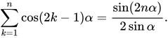
เอกลักษณ์ที่คล้ายกันคือ[ 40 ]
∑ k = 1 n cos ( 2 k − 1 ) α = sin ( 2 n α ) 2 sin α . {\displaystyle \sum _{k=1}^{n}\cos(2k-1)\alpha ={\frac {\sin(2n\alpha )}{2\sin \alpha }}.}
การพิสูจน์มีดังต่อไปนี้ โดยใช้เอกลักษณ์ผลรวมและผลต่างของมุม จาก นั้น ลองพิจารณาสูตรต่อไปนี้sin ( A + B ) − sin ( A − B ) = 2 cos A sin B . {\displaystyle \sin(A+B)-\sin(A-B)=2\cos A\sin B.}
2 sin α ∑ k = 1 n cos ( 2 k − 1 ) α = 2 sin α cos α + 2 sin α cos 3 α + 2 sin α cos 5 α + ⋯ + 2 sin α cos ( 2 n − 1 ) α {\displaystyle 2\sin \alpha \sum _{k=1}^{n}\cos(2k-1)\alpha =2\sin \alpha \cos \alpha +2\sin \alpha \cos 3\alpha +2\sin \alpha \cos 5\alpha +\cdots +2\sin \alpha \cos(2n-1)\alpha }
2 sin α ∑ k = 1 n cos ( 2 k − 1 ) α = ∑ k = 1 n ( sin ( 2 k α ) − sin ( 2 ( k − 1 ) α ) ) = ( sin 2 α − sin 0 ) + ( sin 4 α − sin 2 α ) + ( sin 6 α − sin 4 α ) + ⋯ + ( sin ( 2 n α ) − sin ( 2 ( n − 1 ) α ) ) = sin ( 2 n α ) . {\displaystyle {\begin{aligned}&2\sin \alpha \sum _{k=1}^{n}\cos(2k-1)\alpha \\&\quad =\sum _{k=1}^{n}(\sin(2k\alpha )-\sin(2(k-1)\alpha ))\\&\quad =(\sin 2\alpha -\sin 0)+(\sin 4\alpha -\sin 2\alpha )+(\sin 6\alpha -\sin 4\alpha )+\cdots +(\sin(2n\alpha )-\sin(2(n-1)\alpha ))\\&\quad =\sin(2n\alpha ).\end{aligned}}}
ดังนั้น การหารสูตรนี้ด้วย จึงเป็นการพิสูจน์เสร็จสมบูรณ์2 sin α {\displaystyle 2\sin \alpha }
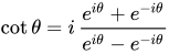
ความสัมพันธ์กับฟังก์ชันไฮเปอร์โบลิกเชิงซ้อน ฟังก์ชันตรีโกณมิติอาจอนุมานได้จากฟังก์ชันไฮเปอร์โบ ลิก ที่มีอาร์กิวเมนต์เชิงซ้อน สูตรสำหรับความสัมพันธ์แสดงไว้ด้านล่าง[ 45 ] [ 46 ] sin x = − i sinh ( i x ) cos x = cosh ( i x ) tan x = − i tanh ( i x ) cot x = i coth ( i x ) sec x = sech ( i x ) csc x = i csch ( i x ) {\displaystyle {\begin{aligned}\sin x&=-i\sinh(ix)\\\cos x&=\cosh(ix)\\\tan x&=-i\tanh(ix)\\\cot x&=i\coth(ix)\\\sec x&=\operatorname {sech} (ix)\\\csc x&=i\operatorname {csch} (ix)\\\end{aligned}}}
การขยายซีรีส์ เมื่อใช้ การขยาย อนุกรมกำลัง เพื่อกำหนดฟังก์ชันตรีโกณมิติ จะได้เอกลักษณ์ต่อไปนี้: [ 47 ]
sin x = x − x 3 3 ! + x 5 5 ! − x 7 7 ! + ⋯ = ∑ n = 0 ∞ ( − 1 ) n x 2 n + 1 ( 2 n + 1 ) ! cos x = 1 − x 2 2 ! + x 4 4 ! − x 6 6 ! + ⋯ = ∑ n = 0 ∞ ( − 1 ) n x 2 n ( 2 n ) ! {\displaystyle {\begin{aligned}\sin x&=x-{\frac {x^{3}}{3!}}+{\frac {x^{5}}{5!}}-{\frac {x^{7}}{7!}}+\cdots &&=\sum _{n=0}^{\infty }(-1)^{n}{\frac {x^{2n+1}}{(2n+1)!}}\\\cos x&=1-{\frac {x^{2}}{2!}}+{\frac {x^{4}}{4!}}-{\frac {x^{6}}{6!}}+\cdots &&=\sum _{n=0}^{\infty }(-1)^{n}{\frac {x^{2n}}{(2n)!}}\end{aligned}}}
สำหรับการประยุกต์ใช้กับฟังก์ชันพิเศษ สูตร ผลคูณอนันต์ ต่อไปนี้สำหรับฟังก์ชันตรีโกณมิติมีประโยชน์: [ 48 ] [ 49 ]
sin x = x ∏ n = 1 ∞ ( 1 − x 2 π 2 n 2 ) , cos x = ∏ n = 1 ∞ ( 1 − x 2 π 2 ( n − 1 2 ) ) 2 ) , sinh x = x ∏ n = 1 ∞ ( 1 + x 2 π 2 n 2 ) , cosh x = ∏ n = 1 ∞ ( 1 + x 2 π 2 ( n − 1 2 ) ) 2 ) . {\displaystyle {\begin{aligned}\sin x&=x\prod _{n=1}^{\infty }\left(1-{\frac {x^{2}}{\pi ^{2}n^{2}}}\right),&\cos x&=\prod _{n=1}^{\infty }\left(1-{\frac {x^{2}}{\pi ^{2}\left(n-{\frac {1}{2}}\right)\!{\vphantom {)}}^{2}}}\right),\\[10mu]\sinh x&=x\prod _{n=1}^{\infty }\left(1+{\frac {x^{2}}{\pi ^{2}n^{2}}}\right),&\cosh x&=\prod _{n=1}^{\infty }\left(1+{\frac {x^{2}}{\pi ^{2}\left(n-{\frac {1}{2}}\right)\!{\vphantom {)}}^{2}}}\right).\end{aligned}}}
ฟังก์ชันตรีโกณมิติผกผัน เอกลักษณ์ต่อไปนี้ให้ผลลัพธ์ของการประกอบฟังก์ชันตรีโกณมิติกับฟังก์ชันตรีโกณมิติผกผัน[ 50 ]
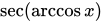
sin ( arcsin x ) = x cos ( arcsin x ) = 1 − x 2 tan ( arcsin x ) = x 1 − x 2 sin ( arccos x ) = 1 − x 2 cos ( arccos x ) = x tan ( arccos x ) = 1 − x 2 x sin ( arctan x ) = x 1 + x 2 cos ( arctan x ) = 1 1 + x 2 tan ( arctan x ) = x sin ( arccsc x ) = 1 x cos ( arccsc x ) = 1 − 1 x 2 tan ( arccsc x ) = 1 x 1 − 1 x 2 sin ( arcsec x ) = 1 − 1 x 2 cos ( arcsec x ) = 1 x tan ( arcsec x ) = x 1 − 1 x 2 sin ( arccot x ) = 1 1 + x 2 cos ( arccot x ) = x 1 + x 2 tan ( arccot x ) = 1 x {\displaystyle {\begin{aligned}\sin(\arcsin x)&=x&\cos(\arcsin x)&={\sqrt {1-x^{2}}}&\tan(\arcsin x)&={\frac {x}{\sqrt {1-x^{2}}}}\\\sin(\arccos x)&={\sqrt {1-x^{2}}}&\cos(\arccos x)&=x&\tan(\arccos x)&={\frac {\sqrt {1-x^{2}}}{x}}\\\sin(\arctan x)&={\frac {x}{\sqrt {1+x^{2}}}}&\cos(\arctan x)&={\frac {1}{\sqrt {1+x^{2}}}}&\tan(\arctan x)&=x\\\sin(\operatorname {arccsc} x)&={\frac {1}{x}}&\cos(\operatorname {arccsc} x)&={\sqrt {1-{\frac {1}{x^{2}}}}}&\tan(\operatorname {arccsc} x)&={\frac {1}{x{\sqrt {1-{\frac {1}{x^{2}}}}}}}\\\sin(\operatorname {arcsec} x)&={\sqrt {1-{\frac {1}{x^{2}}}}}&\cos(\operatorname {arcsec} x)&={\frac {1}{x}}&\tan(\operatorname {arcsec} x)&=x{\sqrt {1-{\frac {1}{x^{2}}}}}\\\sin(\operatorname {arccot} x)&={\frac {1}{\sqrt {1+x^{2}}}}&\cos(\operatorname {arccot} x)&={\frac {x}{\sqrt {1+x^{2}}}}&\tan(\operatorname {arccot} x)&={\frac {1}{x}}\\\end{aligned}}}
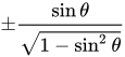
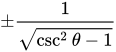
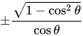
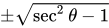
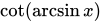
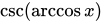
การหาตัวผกผันการคูณ ของทั้งสองข้างของสมการแต่ละสมการข้างต้น จะได้สมการสำหรับ ด้านขวาของสูตรข้างต้นจะถูกพลิกกลับเสมอ ตัวอย่างเช่น สมการสำหรับคือ: ในขณะที่สมการสำหรับและคือ: csc = 1 sin , sec = 1 cos , and cot = 1 tan . {\displaystyle \csc ={\frac {1}{\sin }},\;\sec ={\frac {1}{\cos }},{\text{ and }}\cot ={\frac {1}{\tan }}.} cot ( arcsin x ) {\displaystyle \cot(\arcsin x)} cot ( arcsin x ) = 1 tan ( arcsin x ) = 1 x 1 − x 2 = 1 − x 2 x {\displaystyle \cot(\arcsin x)={\frac {1}{\tan(\arcsin x)}}={\frac {1}{\frac {x}{\sqrt {1-x^{2}}}}}={\frac {\sqrt {1-x^{2}}}{x}}} csc ( arccos x ) {\displaystyle \csc(\arccos x)} sec ( arccos x ) {\displaystyle \sec(\arccos x)} csc ( arccos x ) = 1 sin ( arccos x ) = 1 1 − x 2 and sec ( arccos x ) = 1 cos ( arccos x ) = 1 x . {\displaystyle \csc(\arccos x)={\frac {1}{\sin(\arccos x)}}={\frac {1}{\sqrt {1-x^{2}}}}\qquad {\text{ and }}\quad \sec(\arccos x)={\frac {1}{\cos(\arccos x)}}={\frac {1}{x}}.}
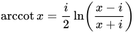
เอกลักษณ์ต่อไปนี้ได้มาจากการอนุมานจากเอกลักษณ์การสะท้อน เอกลักษณ์ เหล่านี้จะเป็นจริงเมื่อใดก็ตามที่และอยู่ในโดเมนของฟังก์ชันที่เกี่ยวข้อง x , r , s , − x , − r , {\displaystyle x,r,s,-x,-r,} − s {\displaystyle -s} π 2 = arcsin ( x ) + arccos ( x ) = arctan ( r ) + arccot ( r ) = arcsec ( s ) + arccsc ( s ) π = arccos ( x ) + arccos ( − x ) = arccot ( r ) + arccot ( − r ) = arcsec ( s ) + arcsec ( − s ) 0 = arcsin ( x ) + arcsin ( − x ) = arctan ( r ) + arctan ( − r ) = arccsc ( s ) + arccsc ( − s ) {\displaystyle {\begin{alignedat}{9}{\frac {\pi }{2}}~&=~\arcsin(x)&&+\arccos(x)~&&=~\arctan(r)&&+\operatorname {arccot}(r)~&&=~\operatorname {arcsec}(s)&&+\operatorname {arccsc}(s)\\[0.4ex]\pi ~&=~\arccos(x)&&+\arccos(-x)~&&=~\operatorname {arccot}(r)&&+\operatorname {arccot}(-r)~&&=~\operatorname {arcsec}(s)&&+\operatorname {arcsec}(-s)\\[0.4ex]0~&=~\arcsin(x)&&+\arcsin(-x)~&&=~\arctan(r)&&+\arctan(-r)~&&=~\operatorname {arccsc}(s)&&+\operatorname {arccsc}(-s)\\[1.0ex]\end{alignedat}}}
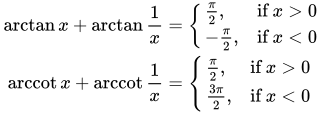
นอกจากนี้[ 51 ] arctan x + arctan 1 x = { π 2 , if x > 0 − π 2 , if x < 0 arccot x + arccot 1 x = { π 2 , if x > 0 3 π 2 , if x < 0 {\displaystyle {\begin{aligned}\arctan x+\arctan {\dfrac {1}{x}}&={\begin{cases}{\frac {\pi }{2}},&{\text{if }}x>0\\-{\frac {\pi }{2}},&{\text{if }}x<0\end{cases}}\\\operatorname {arccot} x+\operatorname {arccot} {\dfrac {1}{x}}&={\begin{cases}{\frac {\pi }{2}},&{\text{if }}x>0\\{\frac {3\pi }{2}},&{\text{if }}x<0\end{cases}}\\\end{aligned}}} arccos 1 x = arcsec x and arcsec 1 x = arccos x {\displaystyle \arccos {\frac {1}{x}}=\operatorname {arcsec} x\qquad {\text{ and }}\qquad \operatorname {arcsec} {\frac {1}{x}}=\arccos x} arcsin 1 x = arccsc x and arccsc 1 x = arcsin x {\displaystyle \arcsin {\frac {1}{x}}=\operatorname {arccsc} x\qquad {\text{ and }}\qquad \operatorname {arccsc} {\frac {1}{x}}=\arcsin x}
ฟังก์ชันอาร์คแทงเจนต์ สามารถขยายเป็นอนุกรมได้ดังนี้: [ 52 ] arctan ( n x ) = ∑ m = 1 n arctan x 1 + ( m − 1 ) m x 2 {\displaystyle \arctan(nx)=\sum _{m=1}^{n}\arctan {\frac {x}{1+(m-1)mx^{2}}}}
เอกลักษณ์ที่ไม่มีตัวแปร ในแง่ของ ฟังก์ชัน อาร์คแทงเจนต์ เรามี[ 51 ] arctan 1 2 = arctan 1 3 + arctan 1 7 {\displaystyle \arctan {\frac {1}{2}}=\arctan {\frac {1}{3}}+\arctan {\frac {1}{7}}}
ซึ่งเป็นกรณีพิเศษของเอกลักษณ์อาร์คแทงเจนต์ของออยเลอร์ [ 53 ]
arctan 1 p = arctan 1 p + q + arctan q p 2 + p q + 1 . {\displaystyle \arctan {\frac {1}{p}}=\arctan {\frac {1}{p+q}}+\arctan {\frac {q}{p^{2}+pq+1}}.}
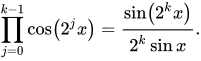
กฎของมอร์รี ซึ่ง เป็นสิ่งที่แปลกประหลาดอย่างยิ่งcos 20 ∘ ⋅ cos 40 ∘ ⋅ cos 80 ∘ = 1 8 , {\displaystyle \cos 20^{\circ }\cdot \cos 40^{\circ }\cdot \cos 80^{\circ }={\frac {1}{8}},}
เป็นกรณีพิเศษของเอกลักษณ์ที่มีตัวแปรเพียงตัวเดียว: ∏ j = 0 k − 1 cos ( 2 j x ) = sin ( 2 k x ) 2 k sin x . {\displaystyle \prod _{j=0}^{k-1}\cos \left(2^{j}x\right)={\frac {\sin \left(2^{k}x\right)}{2^{k}\sin x}}.}
ในทำนองเดียวกัน ถือเป็นกรณีพิเศษของเอกลักษณ์ที่มีลักษณะดังนี้: sin 20 ∘ ⋅ sin 40 ∘ ⋅ sin 80 ∘ = 3 8 {\displaystyle \sin 20^{\circ }\cdot \sin 40^{\circ }\cdot \sin 80^{\circ }={\frac {\sqrt {3}}{8}}} x = 20 ∘ {\displaystyle x=20^{\circ }} sin x ⋅ sin ( 60 ∘ − x ) ⋅ sin ( 60 ∘ + x ) = sin 3 x 4 . {\displaystyle \sin x\cdot \sin \left(60^{\circ }-x\right)\cdot \sin \left(60^{\circ }+x\right)={\frac {\sin 3x}{4}}.}
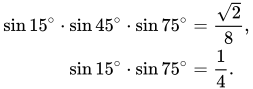
สำหรับกรณีนี้ x = 15 ∘ {\displaystyle x=15^{\circ }} sin 15 ∘ ⋅ sin 45 ∘ ⋅ sin 75 ∘ = 2 8 , sin 15 ∘ ⋅ sin 75 ∘ = 1 4 . {\displaystyle {\begin{aligned}\sin 15^{\circ }\cdot \sin 45^{\circ }\cdot \sin 75^{\circ }&={\frac {\sqrt {2}}{8}},\\\sin 15^{\circ }\cdot \sin 75^{\circ }&={\frac {1}{4}}.\end{aligned}}}
สำหรับกรณีนี้ x = 10 ∘ {\displaystyle x=10^{\circ }} sin 10 ∘ ⋅ sin 50 ∘ ⋅ sin 70 ∘ = 1 8 . {\displaystyle \sin 10^{\circ }\cdot \sin 50^{\circ }\cdot \sin 70^{\circ }={\frac {1}{8}}.}
เอกลักษณ์โคไซน์เดียวกันคือ cos x ⋅ cos ( 60 ∘ − x ) ⋅ cos ( 60 ∘ + x ) = cos 3 x 4 . {\displaystyle \cos x\cdot \cos \left(60^{\circ }-x\right)\cdot \cos \left(60^{\circ }+x\right)={\frac {\cos 3x}{4}}.}
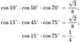
ในทำนองเดียวกัน cos 10 ∘ ⋅ cos 50 ∘ ⋅ cos 70 ∘ = 3 8 , cos 15 ∘ ⋅ cos 45 ∘ ⋅ cos 75 ∘ = 2 8 , cos 15 ∘ ⋅ cos 75 ∘ = 1 4 . {\displaystyle {\begin{aligned}\cos 10^{\circ }\cdot \cos 50^{\circ }\cdot \cos 70^{\circ }&={\frac {\sqrt {3}}{8}},\\\cos 15^{\circ }\cdot \cos 45^{\circ }\cdot \cos 75^{\circ }&={\frac {\sqrt {2}}{8}},\\\cos 15^{\circ }\cdot \cos 75^{\circ }&={\frac {1}{4}}.\end{aligned}}}
ในทำนองเดียวกัน tan 50 ∘ ⋅ tan 60 ∘ ⋅ tan 70 ∘ = tan 80 ∘ , tan 40 ∘ ⋅ tan 30 ∘ ⋅ tan 20 ∘ = tan 10 ∘ . {\displaystyle {\begin{aligned}\tan 50^{\circ }\cdot \tan 60^{\circ }\cdot \tan 70^{\circ }&=\tan 80^{\circ },\\\tan 40^{\circ }\cdot \tan 30^{\circ }\cdot \tan 20^{\circ }&=\tan 10^{\circ }.\end{aligned}}}
ต่อไปนี้เป็นสิ่งที่อาจไม่สามารถนำไปใช้กับเอกลักษณ์ที่มีตัวแปรได้โดยง่ายนัก (แต่โปรดดูคำอธิบายด้านล่าง): cos 24 ∘ + cos 48 ∘ + cos 96 ∘ + cos 168 ∘ = 1 2 . {\displaystyle \cos 24^{\circ }+\cos 48^{\circ }+\cos 96^{\circ }+\cos 168^{\circ }={\frac {1}{2}}.}
หน่วยวัดองศาจะไม่เหมาะสมไปกว่าหน่วยวัดเรเดียนอีกต่อไป เมื่อเราพิจารณาเอกลักษณ์นี้โดยมี 21 อยู่ในตัวส่วน: cos 2 π 21 + cos ( 2 ⋅ 2 π 21 ) + cos ( 4 ⋅ 2 π 21 ) + cos ( 5 ⋅ 2 π 21 ) + cos ( 8 ⋅ 2 π 21 ) + cos ( 10 ⋅ 2 π 21 ) = 1 2 . {\displaystyle \cos {\frac {2\pi }{21}}+\cos \left(2\cdot {\frac {2\pi }{21}}\right)+\cos \left(4\cdot {\frac {2\pi }{21}}\right)+\cos \left(5\cdot {\frac {2\pi }{21}}\right)+\cos \left(8\cdot {\frac {2\pi }{21}}\right)+\cos \left(10\cdot {\frac {2\pi }{21}}\right)={\frac {1}{2}}.}
ตัวประกอบ 1, 2, 4, 5, 8, 10 อาจเริ่มทำให้เห็นรูปแบบได้ชัดเจนขึ้น: พวกมันคือจำนวนเต็มที่น้อยกว่า 21 / 2 ซึ่ง จำนวนเฉพาะสัมพัทธ์ กับ (หรือไม่มีตัวประกอบเฉพาะ ร่วมกับ) 21 ตัวอย่างสุดท้ายหลายตัวอย่างเป็นผลลัพธ์ที่ได้จากข้อเท็จจริงพื้นฐานเกี่ยวกับพหุนามไซโคลโทมิก ที่ไม่สามารถแยกตัวประกอบได้ : ค่าโคไซน์คือส่วนจริงของศูนย์ของพหุนามเหล่านั้น ผลรวมของศูนย์คือฟังก์ชันโมเบียส ที่ประเมินค่าที่ (ในกรณีสุดท้ายข้างต้น) 21 มีเพียงครึ่งหนึ่งของศูนย์เท่านั้นที่ปรากฏอยู่ข้างต้น เอกลักษณ์ที่อยู่ก่อนหน้าอันสุดท้ายนี้เกิดขึ้นในลักษณะเดียวกันโดยแทนที่ 21 ด้วย 15
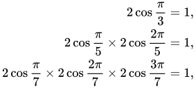
เอกลักษณ์โคไซน์อื่นๆ ได้แก่[ 54 ] 2 cos π 3 = 1 , 2 cos π 5 × 2 cos 2 π 5 = 1 , 2 cos π 7 × 2 cos 2 π 7 × 2 cos 3 π 7 = 1 , {\displaystyle {\begin{aligned}2\cos {\frac {\pi }{3}}&=1,\\2\cos {\frac {\pi }{5}}\times 2\cos {\frac {2\pi }{5}}&=1,\\2\cos {\frac {\pi }{7}}\times 2\cos {\frac {2\pi }{7}}\times 2\cos {\frac {3\pi }{7}}&=1,\end{aligned}}} cos π 3 + cos π 5 × cos 2 π 5 + cos π 7 × cos 2 π 7 × cos 3 π 7 + ⋯ = 1. {\displaystyle \cos {\frac {\pi }{3}}+\cos {\frac {\pi }{5}}\times \cos {\frac {2\pi }{5}}+\cos {\frac {\pi }{7}}\times \cos {\frac {2\pi }{7}}\times \cos {\frac {3\pi }{7}}+\dots =1.}
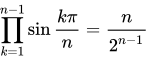
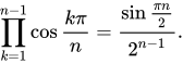
อัตลักษณ์ที่น่าสนใจเหล่านั้นจำนวนมากมีที่มาจากข้อเท็จจริงทั่วไปดังต่อไปนี้: [ 55 ] ∏ k = 1 n − 1 sin k π n = n 2 n − 1 {\displaystyle \prod _{k=1}^{n-1}\sin {\frac {k\pi }{n}}={\frac {n}{2^{n-1}}}} ∏ k = 1 n − 1 cos k π n = sin π n 2 2 n − 1 . {\displaystyle \prod _{k=1}^{n-1}\cos {\frac {k\pi }{n}}={\frac {\sin {\frac {\pi n}{2}}}{2^{n-1}}}.}
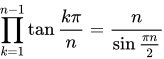
เมื่อนำสิ่งเหล่านี้มารวมกันจะได้ผลลัพธ์ดังนี้ ∏ k = 1 n − 1 tan k π n = n sin π n 2 {\displaystyle \prod _{k=1}^{n-1}\tan {\frac {k\pi }{n}}={\frac {n}{\sin {\frac {\pi n}{2}}}}}
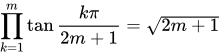
ถ้าn เป็นจำนวนคี่ ( ) เราสามารถใช้สมมาตรเพื่อให้ได้ n = 2 m + 1 {\displaystyle n=2m+1} ∏ k = 1 m tan k π 2 m + 1 = 2 m + 1 {\displaystyle \prod _{k=1}^{m}\tan {\frac {k\pi }{2m+1}}={\sqrt {2m+1}}}
ฟังก์ชันถ่ายโอนของตัวกรองความถี่ต่ำแบบ Butterworth สามารถแสดงได้ในรูปของพหุนามและขั้ว โดยการกำหนดความถี่เป็นความถี่ตัด จะสามารถพิสูจน์เอกลักษณ์ต่อไปนี้ได้: ∏ k = 1 n sin ( 2 k − 1 ) π 4 n = ∏ k = 1 n cos ( 2 k − 1 ) π 4 n = 2 2 n {\displaystyle \prod _{k=1}^{n}\sin {\frac {\left(2k-1\right)\pi }{4n}}=\prod _{k=1}^{n}\cos {\frac {\left(2k-1\right)\pi }{4n}}={\frac {\sqrt {2}}{2^{n}}}}
π วิธีที่มีประสิทธิภาพในการคำนวณค่าπ ให้ได้จำนวนหลักจำนวนมาก นั้น ใช้สูตรเอกลักษณ์แบบไม่มีตัวแปรของMachin ดังต่อไป นี้ ซึ่งเรียกว่าสูตรแบบ Machin : หรืออีกวิธีหนึ่งคือใช้สูตรเอกลักษณ์ของLeonhard Euler : หรือโดยใช้สามเหลี่ยมพีทาโกเรียน : π 4 = 4 arctan 1 5 − arctan 1 239 {\displaystyle {\frac {\pi }{4}}=4\arctan {\frac {1}{5}}-\arctan {\frac {1}{239}}} π 4 = 5 arctan 1 7 + 2 arctan 3 79 {\displaystyle {\frac {\pi }{4}}=5\arctan {\frac {1}{7}}+2\arctan {\frac {3}{79}}} π = arccos 4 5 + arccos 5 13 + arccos 16 65 = arcsin 3 5 + arcsin 12 13 + arcsin 63 65 . {\displaystyle \pi =\arccos {\frac {4}{5}}+\arccos {\frac {5}{13}}+\arccos {\frac {16}{65}}=\arcsin {\frac {3}{5}}+\arcsin {\frac {12}{13}}+\arcsin {\frac {63}{65}}.}
อื่นๆ ได้แก่: [ 56 ] [ 51 ] π 4 = arctan 1 2 + arctan 1 3 , {\displaystyle {\frac {\pi }{4}}=\arctan {\frac {1}{2}}+\arctan {\frac {1}{3}},} π = arctan 1 + arctan 2 + arctan 3 , {\displaystyle \pi =\arctan 1+\arctan 2+\arctan 3,} π 4 = 2 arctan 1 3 + arctan 1 7 . {\displaystyle {\frac {\pi }{4}}=2\arctan {\frac {1}{3}}+\arctan {\frac {1}{7}}.}
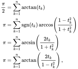
Generally, for numbers t , ..., t ∈ (−1, 1)θ = Σn −1t ∈ (π /4, 3π /4)t = tan(π /2 − θ ) = cot θ t , ..., t (−1, 1) . In particular, the computed t t , ..., t π 2 = ∑ k = 1 n arctan ( t k ) π = ∑ k = 1 n sgn ( t k ) arccos ( 1 − t k 2 1 + t k 2 ) π = ∑ k = 1 n arcsin ( 2 t k 1 + t k 2 ) π = ∑ k = 1 n arctan ( 2 t k 1 − t k 2 ) , {\displaystyle {\begin{aligned}{\frac {\pi }{2}}&=\sum _{k=1}^{n}\arctan(t_{k})\\\pi &=\sum _{k=1}^{n}\operatorname {sgn}(t_{k})\arccos \left({\frac {1-t_{k}^{2}}{1+t_{k}^{2}}}\right)\\\pi &=\sum _{k=1}^{n}\arcsin \left({\frac {2t_{k}}{1+t_{k}^{2}}}\right)\\\pi &=\sum _{k=1}^{n}\arctan \left({\frac {2t_{k}}{1-t_{k}^{2}}}\right)\,,\end{aligned}}}
where in all but the first expression, we have used tangent half-angle formulae. The first two formulae work even if one or more of the t (−1, 1) . Note that if t = p /q (2t , 1 − t 2 , 1 + t 2 ) values in the above formulae are proportional to the Pythagorean triple (2pq , q 2 − p 2 , q 2 + p 2 ) .
For example, for n = 3π 2 = arctan ( a b ) + arctan ( c d ) + arctan ( b d − a c a d + b c ) {\displaystyle {\frac {\pi }{2}}=\arctan \left({\frac {a}{b}}\right)+\arctan \left({\frac {c}{d}}\right)+\arctan \left({\frac {bd-ac}{ad+bc}}\right)} a , b , c , d > 0
An identity of Euclid Euclid showed in Book XIII, Proposition 10 of his Elements sin 2 18 ∘ + sin 2 30 ∘ = sin 2 36 ∘ . {\displaystyle \sin ^{2}18^{\circ }+\sin ^{2}30^{\circ }=\sin ^{2}36^{\circ }.}
Ptolemy used this proposition to compute some angles in his table of chords in Book I, chapter 11 of Almagest
Composition of trigonometric functions These identities involve a trigonometric function of a trigonometric function:[ 57]
cos ( t sin x ) = J 0 ( t ) + 2 ∑ k = 1 ∞ J 2 k ( t ) cos ( 2 k x ) {\displaystyle \cos(t\sin x)=J_{0}(t)+2\sum _{k=1}^{\infty }J_{2k}(t)\cos(2kx)} sin ( t sin x ) = 2 ∑ k = 0 ∞ J 2 k + 1 ( t ) sin ( ( 2 k + 1 ) x ) {\displaystyle \sin(t\sin x)=2\sum _{k=0}^{\infty }J_{2k+1}(t)\sin {\big (}(2k+1)x{\big )}} cos ( t cos x ) = J 0 ( t ) + 2 ∑ k = 1 ∞ ( − 1 ) k J 2 k ( t ) cos ( 2 k x ) {\displaystyle \cos(t\cos x)=J_{0}(t)+2\sum _{k=1}^{\infty }(-1)^{k}J_{2k}(t)\cos(2kx)} sin ( t cos x ) = 2 ∑ k = 0 ∞ ( − 1 ) k J 2 k + 1 ( t ) cos ( ( 2 k + 1 ) x ) {\displaystyle \sin(t\cos x)=2\sum _{k=0}^{\infty }(-1)^{k}J_{2k+1}(t)\cos {\big (}(2k+1)x{\big )}} where J are Bessel functions .
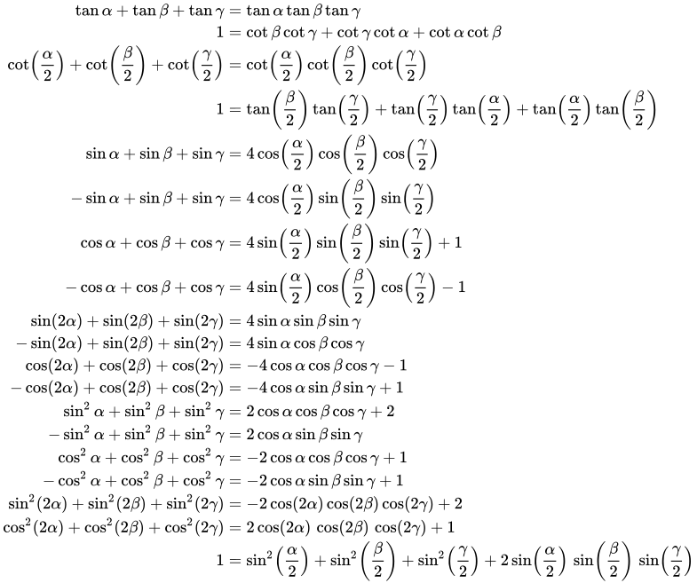
α + β + γ = 180°A conditional trigonometric identity is a trigonometric identity that holds if specified conditions on the arguments to the trigonometric functions are satisfied.[ 58] α + β + γ = 180 ∘ , {\displaystyle \alpha +\beta +\gamma =180^{\circ },} [ 59] tan α + tan β + tan γ = tan α tan β tan γ 1 = cot β cot γ + cot γ cot α + cot α cot β cot ( α 2 ) + cot ( β 2 ) + cot ( γ 2 ) = cot ( α 2 ) cot ( β 2 ) cot ( γ 2 ) 1 = tan ( β 2 ) tan ( γ 2 ) + tan ( γ 2 ) tan ( α 2 ) + tan ( α 2 ) tan ( β 2 ) sin α + sin β + sin γ = 4 cos ( α 2 ) cos ( β 2 ) cos ( γ 2 ) − sin α + sin β + sin γ = 4 cos ( α 2 ) sin ( β 2 ) sin ( γ 2 ) cos α + cos β + cos γ = 4 sin ( α 2 ) sin ( β 2 ) sin ( γ 2 ) + 1 − cos α + cos β + cos γ = 4 sin ( α 2 ) cos ( β 2 ) cos ( γ 2 ) − 1 sin ( 2 α ) + sin ( 2 β ) + sin ( 2 γ ) = 4 sin α sin β sin γ − sin ( 2 α ) + sin ( 2 β ) + sin ( 2 γ ) = 4 sin α cos β cos γ cos ( 2 α ) + cos ( 2 β ) + cos ( 2 γ ) = − 4 cos α cos β cos γ − 1 − cos ( 2 α ) + cos ( 2 β ) + cos ( 2 γ ) = − 4 cos α sin β sin γ + 1 sin 2 α + sin 2 β + sin 2 γ = 2 cos α cos β cos γ + 2 − sin 2 α + sin 2 β + sin 2 γ = 2 cos α sin β sin γ cos 2 α + cos 2 β + cos 2 γ = − 2 cos α cos β cos γ + 1 − cos 2 α + cos 2 β + cos 2 γ = − 2 cos α sin β sin γ + 1 sin 2 ( 2 α ) + sin 2 ( 2 β ) + sin 2 ( 2 γ ) = − 2 cos ( 2 α ) cos ( 2 β ) cos ( 2 γ ) + 2 cos 2 ( 2 α ) + cos 2 ( 2 β ) + cos 2 ( 2 γ ) = 2 cos ( 2 α ) cos ( 2 β ) cos ( 2 γ ) + 1 1 = sin 2 ( α 2 ) + sin 2 ( β 2 ) + sin 2 ( γ 2 ) + 2 sin ( α 2 ) sin ( β 2 ) sin ( γ 2 ) {\displaystyle {\begin{aligned}\tan \alpha +\tan \beta +\tan \gamma &=\tan \alpha \tan \beta \tan \gamma \\1&=\cot \beta \cot \gamma +\cot \gamma \cot \alpha +\cot \alpha \cot \beta \\\cot \left({\frac {\alpha }{2}}\right)+\cot \left({\frac {\beta }{2}}\right)+\cot \left({\frac {\gamma }{2}}\right)&=\cot \left({\frac {\alpha }{2}}\right)\cot \left({\frac {\beta }{2}}\right)\cot \left({\frac {\gamma }{2}}\right)\\1&=\tan \left({\frac {\beta }{2}}\right)\tan \left({\frac {\gamma }{2}}\right)+\tan \left({\frac {\gamma }{2}}\right)\tan \left({\frac {\alpha }{2}}\right)+\tan \left({\frac {\alpha }{2}}\right)\tan \left({\frac {\beta }{2}}\right)\\\sin \alpha +\sin \beta +\sin \gamma &=4\cos \left({\frac {\alpha }{2}}\right)\cos \left({\frac {\beta }{2}}\right)\cos \left({\frac {\gamma }{2}}\right)\\-\sin \alpha +\sin \beta +\sin \gamma &=4\cos \left({\frac {\alpha }{2}}\right)\sin \left({\frac {\beta }{2}}\right)\sin \left({\frac {\gamma }{2}}\right)\\\cos \alpha +\cos \beta +\cos \gamma &=4\sin \left({\frac {\alpha }{2}}\right)\sin \left({\frac {\beta }{2}}\right)\sin \left({\frac {\gamma }{2}}\right)+1\\-\cos \alpha +\cos \beta +\cos \gamma &=4\sin \left({\frac {\alpha }{2}}\right)\cos \left({\frac {\beta }{2}}\right)\cos \left({\frac {\gamma }{2}}\right)-1\\\sin(2\alpha )+\sin(2\beta )+\sin(2\gamma )&=4\sin \alpha \sin \beta \sin \gamma \\-\sin(2\alpha )+\sin(2\beta )+\sin(2\gamma )&=4\sin \alpha \cos \beta \cos \gamma \\\cos(2\alpha )+\cos(2\beta )+\cos(2\gamma )&=-4\cos \alpha \cos \beta \cos \gamma -1\\-\cos(2\alpha )+\cos(2\beta )+\cos(2\gamma )&=-4\cos \alpha \sin \beta \sin \gamma +1\\\sin ^{2}\alpha +\sin ^{2}\beta +\sin ^{2}\gamma &=2\cos \alpha \cos \beta \cos \gamma +2\\-\sin ^{2}\alpha +\sin ^{2}\beta +\sin ^{2}\gamma &=2\cos \alpha \sin \beta \sin \gamma \\\cos ^{2}\alpha +\cos ^{2}\beta +\cos ^{2}\gamma &=-2\cos \alpha \cos \beta \cos \gamma +1\\-\cos ^{2}\alpha +\cos ^{2}\beta +\cos ^{2}\gamma &=-2\cos \alpha \sin \beta \sin \gamma +1\\\sin ^{2}(2\alpha )+\sin ^{2}(2\beta )+\sin ^{2}(2\gamma )&=-2\cos(2\alpha )\cos(2\beta )\cos(2\gamma )+2\\\cos ^{2}(2\alpha )+\cos ^{2}(2\beta )+\cos ^{2}(2\gamma )&=2\cos(2\alpha )\,\cos(2\beta )\,\cos(2\gamma )+1\\1&=\sin ^{2}\left({\frac {\alpha }{2}}\right)+\sin ^{2}\left({\frac {\beta }{2}}\right)+\sin ^{2}\left({\frac {\gamma }{2}}\right)+2\sin \left({\frac {\alpha }{2}}\right)\,\sin \left({\frac {\beta }{2}}\right)\,\sin \left({\frac {\gamma }{2}}\right)\end{aligned}}}
Miscellaneous
Dirichlet kernel The Dirichlet kernel D (x )1 + 2 cos x + 2 cos ( 2 x ) + 2 cos ( 3 x ) + ⋯ + 2 cos ( n x ) = sin ( ( n + 1 2 ) x ) sin ( 1 2 x ) . {\displaystyle 1+2\cos x+2\cos(2x)+2\cos(3x)+\cdots +2\cos(nx)={\frac {\sin \left(\left(n+{\frac {1}{2}}\right)x\right)}{\sin \left({\frac {1}{2}}x\right)}}.}
The convolution of any integrable function of period 2 π {\displaystyle 2\pi } n {\displaystyle n} measure or generalized function .
cos θ 2 ⋅ cos θ 4 ⋅ cos θ 8 ⋯ = ∏ n = 1 ∞ cos θ 2 n = sin θ θ = sinc θ . {\displaystyle \cos {\frac {\theta }{2}}\cdot \cos {\frac {\theta }{4}}\cdot \cos {\frac {\theta }{8}}\cdots =\prod _{n=1}^{\infty }\cos {\frac {\theta }{2^{n}}}={\frac {\sin \theta }{\theta }}=\operatorname {sinc} \theta .}
A sine identity used in medical imaging Here is an identity discovered as a by-product of research in medical imaging .[ 61]
Let i = − 1 {\displaystyle i={\sqrt {-1}}} ∘ denote composition of differential operators. Then for every odd positive integer n ,
∑ k = 0 n ( n k ) ( d d x − sin x ) ∘ ( d d x − sin x + i ) ∘ ⋯ ⋯ ∘ ( d d x − sin x + ( k − 1 ) i ) ( sin x ) n − k = 0. {\displaystyle {\begin{aligned}\sum _{k=0}^{n}{\binom {n}{k}}\left({\frac {d}{dx}}-\sin x\right)&\circ \left({\frac {d}{dx}}-\sin x+i\right)\circ \cdots \\\cdots &\circ \left({\frac {d}{dx}}-\sin x+(k-1)i\right)(\sin x)^{n-k}=0.\end{aligned}}} (When k = 0, then the number of differential operators being composed is 0, so the corresponding term in the sum above is just (sin x )n .)
Bibliography Abramowitz, Milton ; Stegun, Irene A. , eds. (1972). Handbook of Mathematical Functions with Formulas, Graphs, and Mathematical Tables . New York: Dover Publications . ISBN 978-0-486-61272-0 .Nielsen, Kaj L. (1966), Logarithmic and Trigonometric Tables to Five Places (2nd ed.), New York: Barnes & Noble , LCCN 61-9103 Selby, Samuel M., ed. (1970), Standard Mathematical Tables (18th ed.), The Chemical Rubber Co.
External links Values of sin and cos, expressed in surds, for integer multiples of 3° and of 5+ 5 / 8 

































































![{\displaystyle {\begin{aligned}\operatorname {sgn} (\sin \theta )=\operatorname {sgn} (\csc \theta )&={\begin{cases}+1&{\text{ถ้า}}\ \ 0<\theta <\pi \\-1&{\text{ถ้า}}\ \ {-\pi }<\theta <0\\0&{\text{ถ้า}}\ \ \theta \in \{0,\pi \}\end{cases}}\\[5mu]\operatorname {sgn} (\cos \theta )=\operatorname {sgn} (\sec \theta )&={\begin{cases}+1&{\text{ถ้า}}\ \ {-{\tfrac {\pi }{2}}}<\theta <{\tfrac {\pi }{2}}\\-1&{\text{ถ้า}}\ \ {-\pi }<\theta <-{\tfrac {\pi }{2}}\ \ {\text{หรือ}}\ \ {\tfrac {\pi }{2}}<\theta <\pi \\0&{\text{ถ้า}}\ \ \theta \in {\bigl \{}{-{\tfrac {\pi }{2}}},{\tfrac {\pi }{2}}{\bigr \}}\end{cases}}\\[5mu]\operatorname {sgn} (\tan \theta )=\operatorname {sgn} (\cot \theta )&={\begin{cases}+1&{\text{ถ้า}}\ \ {-\pi }<\theta <-{\tfrac {\pi }{2}}\ \ {\text{หรือ}}\ \ 0<\theta <{\tfrac {\pi }{2}}\\-1&{\text{ถ้า}}\ \ {-{\tfrac {\pi }{2}}}<\theta <0\ \ {\text{หรือ}}\ \ {\tfrac {\pi }{2}}<\theta <\pi \\0&{\text{ถ้า}}\ \ \theta \in {\bigl \{}{-{\tfrac {\pi }{2}}},0,{\tfrac {\pi }{2}},\pi {\bigr \}}\end{cases}}\end{aligned}}}](https://wikimedia.org/api/rest_v1/media/math/render/svg/3885aee3a70a73da0b369ad2f21a8122f4e78587)

![{\displaystyle ({-\pi },\pi ],}](https://wikimedia.org/api/rest_v1/media/math/render/svg/122328145a5f3a4162d21b4fbb5f4d1149932d2b)































![{\displaystyle {\begin{aligned}e_{0}&=1\\[6pt]e_{1}&=\sum _{i}x_{i}&&=\sum _{i}\tan \theta _{i}\\[6pt]e_{2}&=\sum _{i<j}x_{i}x_{j}&&=\sum _{i<j}\tan \theta _{i}\tan \theta _{j}\\[6pt]e_{3}&=\sum _{i<j<k}x_{i}x_{j}x_{k}&&=\sum _{i<j<k}\tan \theta _{i}\tan \theta _{j}\tan \theta _{k}\\&\ \ \vdots &&\ \ \vdots \end{aligned}}}](https://wikimedia.org/api/rest_v1/media/math/render/svg/cb1927ae2be96f5156e18813a20486fdb0ff72f1)

![{\displaystyle {\begin{aligned}\tan {\Bigl (}\sum _{i}\theta _{i}{\Bigr )}&={\frac {{\sin }{\bigl (}\sum _{i}\theta _{i}{\bigr )}/\prod _{i}\cos \theta _{i}}{{\cos }{\bigl (}\sum _{i}\theta _{i}{\bigr )}/\prod _{i}\cos \theta _{i}}}\\[10pt]&={\frac {\displaystyle \sum _{{\text{odd}}\ k\geq 1}(-1)^{\frac {k-1}{2}}\sum _{\begin{smallmatrix}A\subseteq \{1,2,3,\dots \}\\\left|A\right|=k\end{smallmatrix}}\prod _{i\in A}\tan \theta _{i}}{\displaystyle \sum _{{\text{even}}\ k\geq 0}~(-1)^{\frac {k}{2}}~~\sum _{\begin{smallmatrix}A\subseteq \{1,2,3,\dots \}\\\left|A\right|=k\end{smallmatrix}}\prod _{i\in A}\tan \theta _{i}}}={\frac {e_{1}-e_{3}+e_{5}-\cdots }{e_{0}-e_{2}+e_{4}-\cdots }}\\[10pt]\cot {\Bigl (}\sum _{i}\theta _{i}{\Bigr )}&={\frac {e_{0}-e_{2}+e_{4}-\cdots }{e_{1}-e_{3}+e_{5}-\cdots }}\end{aligned}}}](https://wikimedia.org/api/rest_v1/media/math/render/svg/55ff3a24e1e073c731c170651eca41efdad72212)
![{\displaystyle {\begin{aligned}\tan(\theta _{1}+\theta _{2})&={\frac {e_{1}}{e_{0}-e_{2}}}={\frac {x_{1}+x_{2}}{1\ -\ x_{1}x_{2}}}={\frac {\tan \theta _{1}+\tan \theta _{2}}{1\ -\ \tan \theta _{1}\tan \theta _{2}}},\\[8pt]\tan(\theta _{1}+\theta _{2}+\theta _{3})&={\frac {e_{1}-e_{3}}{e_{0}-e_{2}}}={\frac {(x_{1}+x_{2}+x_{3})\ -\ (x_{1}x_{2}x_{3})}{1\ -\ (x_{1}x_{2}+x_{1}x_{3}+x_{2}x_{3})}},\\[8pt]\tan(\theta _{1}+\theta _{2}+\theta _{3}+\theta _{4})&={\frac {e_{1}-e_{3}}{e_{0}-e_{2}+e_{4}}}\\[8pt]&={\frac {(x_{1}+x_{2}+x_{3}+x_{4})\ -\ (x_{1}x_{2}x_{3}+x_{1}x_{2}x_{4}+x_{1}x_{3}x_{4}+x_{2}x_{3}x_{4})}{1\ -\ (x_{1}x_{2}+x_{1}x_{3}+x_{1}x_{4}+x_{2}x_{3}+x_{2}x_{4}+x_{3}x_{4})\ +\ (x_{1}x_{2}x_{3}x_{4})}},\end{aligned}}}](https://wikimedia.org/api/rest_v1/media/math/render/svg/4c9196b8ab5e0aef6cf7d7fec7d7546f2a6e7d2f)


![{\displaystyle {\begin{aligned}{\sec }{\Bigl (}\sum _{i}\theta _{i}{\Bigr )}&={\frac {\prod _{i}\sec \theta _{i}}{e_{0}-e_{2}+e_{4}-\cdots }}\\[8pt]{\csc }{\Bigl (}\sum _{i}\theta _{i}{\Bigr )}&={\frac {\prod _{i}\sec \theta _{i}}{e_{1}-e_{3}+e_{5}-\cdots }}\end{aligned}}}](https://wikimedia.org/api/rest_v1/media/math/render/svg/b24f2b169fbe11608507c63f5bb728e03b2b4957)


![{\displaystyle {\begin{aligned}\sec(\alpha +\beta +\gamma )&={\frac {\sec \alpha \sec \beta \sec \gamma }{1-\tan \alpha \tan \beta -\tan \alpha \tan \gamma -\tan \beta \tan \gamma }}\\[8pt]\csc(\alpha +\beta +\gamma )&={\frac {\sec \alpha \sec \beta \sec \gamma }{\tan \alpha +\tan \beta +\tan \gamma -\tan \alpha \tan \beta \tan \gamma }}.\end{aligned}}}](https://wikimedia.org/api/rest_v1/media/math/render/svg/e082e69aab7a9c782f590f3a93262ba3101899b7)















![{\displaystyle {\begin{aligned}\sin {\frac {\theta }{2}}&=\operatorname {sgn} \left(\sin {\frac {\theta }{2}}\right){\sqrt {\frac {1-\cos \theta }{2}}}\\[3pt]\cos {\frac {\theta }{2}}&=\operatorname {sgn} \left(\cos {\frac {\theta }{2}}\right){\sqrt {\frac {1+\cos \theta }{2}}}\\[3pt]\tan {\frac {\theta }{2}}&={\frac {1-\cos \theta }{\sin \theta }}={\frac {\sin \theta }{1+\cos \theta }}=\csc \theta -\cot \theta ={\frac {\tan \theta }{1+\sec {\theta }}}\\[6mu]&=\operatorname {sgn} (\sin \theta ){\sqrt {\frac {1-\cos \theta }{1+\cos \theta }}}={\frac {-1+\operatorname {sgn} (\cos \theta ){\sqrt {1+\tan ^{2}\theta }}}{\tan \theta }}\\[3pt]\cot {\frac {\theta }{2}}&={\frac {1+\cos \theta }{\sin \theta }}={\frac {\sin \theta }{1-\cos \theta }}=\csc \theta +\cot \theta =\operatorname {sgn} (\sin \theta ){\sqrt {\frac {1+\cos \theta }{1-\cos \theta }}}\\\sec {\frac {\theta }{2}}&=\operatorname {sgn} \left(\cos {\frac {\theta }{2}}\right){\sqrt {\frac {2}{1+\cos \theta }}}\\\csc {\frac {\theta }{2}}&=\operatorname {sgn} \left(\sin {\frac {\theta }{2}}\right){\sqrt {\frac {2}{1-\cos \theta }}}\\\end{aligned}}}](https://wikimedia.org/api/rest_v1/media/math/render/svg/d53d104c73c4b28f1dd7bfa5d2b0c7207c68cd87)
![{\displaystyle {\begin{aligned}\tan {\frac {\eta \pm \theta }{2}}&={\frac {\sin \eta \pm \sin \theta }{\cos \eta +\cos \theta }}\\[3pt]\tan \left({\frac {\theta }{2}}+{\frac {\pi }{4}}\right)&=\sec \theta +\tan \theta \\[3pt]{\sqrt {\frac {1-\sin \theta }{1+\sin \theta }}}&={\frac {\left|1-\tan {\frac {\theta }{2}}\right|}{\left|1+\tan {\frac {\theta }{2}}\right|}}\end{aligned}}}](https://wikimedia.org/api/rest_v1/media/math/render/svg/639270245e163f1afa8682ac8aa12086db43dce1)


![{\displaystyle {\begin{aligned}\tan {\frac {\theta }{2}}&=\csc \theta -\cot \theta \\&=\pm \,{\sqrt {\frac {1-\cos \theta }{1+\cos \theta }}}\\[3pt]&={\frac {\sin \theta }{1+\cos \theta }}\\[3pt]&={\frac {1-\cos \theta }{\sin \theta }}\\[5pt]\tan {\frac {\eta +\theta }{2}}&={\frac {\sin \eta +\sin \theta }{\cos \eta +\cos \theta }}\\[5pt]\tan \left({\frac {\theta }{2}}+{\frac {\pi }{4}}\right)&=\sec \theta +\tan \theta \\[5pt]{\sqrt {\frac {1-\sin \theta }{1+\sin \theta }}}&={\frac {\left|1-\tan {\frac {\theta }{2}}\right|}{\left|1+\tan {\frac {\theta }{2}}\right|}}\\[5pt]\tan {\frac {\theta }{2}}&={\frac {\tan \theta }{1+{\sqrt {1+\tan ^{2}\theta }}}}\\&{\text{สำหรับ }}\theta \in \left(-{\tfrac {\pi }{2}},{\tfrac {\pi }{2}}\right)\end{aligned}}}](https://wikimedia.org/api/rest_v1/media/math/render/svg/3cab50a58d64b8c3341fb4f7646888bbbc67ea0c)
![{\displaystyle {\begin{aligned}\cot {\frac {\theta }{2}}&=\csc \theta +\cot \theta \\&=\pm \,{\sqrt {\frac {1+\cos \theta }{1-\cos \theta }}}\\[3pt]&={\frac {\sin \theta }{1-\cos \theta }}\\[4pt]&={\frac {1+\cos \theta }{\sin \theta }}\end{aligned}}}](https://wikimedia.org/api/rest_v1/media/math/render/svg/5c9be831a310f112ffc6e5790bc705dc7b070b87)











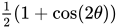












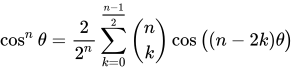




![{\displaystyle {\begin{aligned}\cos \theta \,\cos \varphi &={\tfrac {1}{2}}{\bigl (}\!\!~\cos(\theta -\varphi )+\cos(\theta +\varphi ){\bigr )},\\[5mu]\sin \theta \,\sin \varphi &={\tfrac {1}{2}}{\bigl (}\!\!~\cos(\theta -\varphi )-\cos(\theta +\varphi ){\bigr )},\\[5mu]\sin \theta \,\cos \varphi &={\tfrac {1}{2}}{\bigl (}\!\!~\sin(\theta +\varphi )+\sin(\theta -\varphi ){\bigr )},\\[5mu]\cos \theta \,\sin \varphi &={\tfrac {1}{2}}{\bigl (}\!\!~\sin(\theta +\varphi )-\sin(\theta -\varphi ){\bigr )}.\end{aligned}}}](https://wikimedia.org/api/rest_v1/media/math/render/svg/dcd715f4b6380798a701537d9c067f28cc371efa)
![{\displaystyle {\begin{aligned}\tan \theta \,\tan \varphi &={\frac {\cos(\theta -\varphi )-\cos(\theta +\varphi )}{\cos(\theta -\varphi )+\cos(\theta +\varphi )}},\\[5mu]{\frac {\tan \theta }{\tan \varphi }}&={\frac {\sin(\theta +\varphi )+\sin(\theta -\varphi )}{\sin(\theta +\varphi )-\sin(\theta -\varphi )}}.\end{aligned}}}](https://wikimedia.org/api/rest_v1/media/math/render/svg/69a3a5dee2394b1ed85551729df20f0abd6770b7)
![{\displaystyle {\begin{aligned}\prod _{k=1}^{n}\cos \theta _{k}&={\frac {1}{2^{n}}}\sum _{e\in S}\cos(e_{1}\theta _{1}+\cdots +e_{n}\theta _{n})\\[5mu]&{\text{where }}e=(e_{1},\ldots ,e_{n})\in S=\{1,-1\}^{n},\\\prod _{k=1}^{n}\sin \theta _{k}&={\frac {(-1)^{\left\lfloor {\frac {n}{2}}\right\rfloor }}{2^{n}}}{\begin{cases}\displaystyle \sum _{e\in \begin{aligned}}} \cos(e_{1}\theta _{1}+\cdots +e_{n}\theta _{n})\prod _{j=1}^{n}e_{j}\;{\text{ถ้า}}\;n\;{\text{เป็นจำนวนคู่}},\\\displaystyle \sum _{e\in S}\sin(e_{1}\theta _{1}+\cdots +e_{n}\theta _{n})\prod _{j=1}^{n}e_{j}\;{\text{ถ้า}}\;n\;{\text{เป็นจำนวนคี่}}.\end{cases}}\end{aligned}}}](https://wikimedia.org/api/rest_v1/media/math/render/svg/106ce6115e77f036a95a2096bc66b01927e5dff9)


![{\displaystyle {\begin{aligned}\sin \theta +\sin \varphi &=2\sin {\tfrac {1}{2}}(\theta +\varphi )\,\cos {\tfrac {1}{2}}(\theta -\varphi ),\\[5mu]\sin \theta -\sin \varphi &=2\cos {\tfrac {1}{2}}(\theta +\varphi )\,\sin {\tfrac {1}{2}}(\theta -\varphi ),\\[5mu]\cos \theta +\cos \varphi &=2\cos {\tfrac {1}{2}}(\theta +\varphi )\,\cos {\tfrac {1}{2}}(\theta -\varphi ),\\[5mu]\cos \theta -\cos \varphi &=-2\sin {\tfrac {1}{2}}(\ทีต้า +\varphi )\,\sin {\tfrac {1}{2}}(\theta -\varphi ).\end{aligned}}}](https://wikimedia.org/api/rest_v1/media/math/render/svg/3676cbeab42be735d5fb198d843eeec23ee9b763)













![{\displaystyle {\begin{aligned}\sum _{k=0}^{n}\sin k\theta &={\frac {\cos {\tfrac {1}{2}}\theta -\cos \left(\left(n+{\tfrac {1}{2}}\right)\theta \right)}{2\sin {\tfrac {1}{2}}\theta }}\\[5pt]\sum _{k=1}^{n}\cos k\theta &={\frac {-\sin {\tfrac {1}{2}}\theta +\sin \left(\left(n+{\tfrac {1}{2}}\right)\theta \right)}{2\sin {\tfrac {1}{2}}\theta }}\end{aligned}}}](https://wikimedia.org/api/rest_v1/media/math/render/svg/4679d7bb8112018d06e7d3a849bbe4ce024ff148)










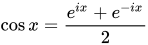
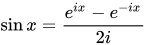
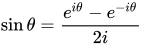

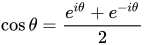

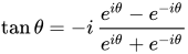
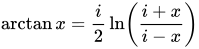
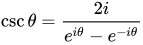

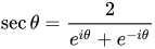





![{\displaystyle {\begin{aligned}\sin x&=x\prod _{n=1}^{\infty }\left(1-{\frac {x^{2}}{\pi ^{2}n^{2}}}\right),&\cos x&=\prod _{n=1}^{\infty }\left(1-{\frac {x^{2}}{\pi ^{2}\left(n-{\frac {1}{2}}\right)\!{\vphantom {)}}^{2}}}\right),\\[10mu]\sinh x&=x\prod _{n=1}^{\infty }\left(1+{\frac {x^{2}}{\pi ^{2}n^{2}}}\right),&\cosh x&=\prod _{n=1}^{\infty }\left(1+{\frac {x^{2}}{\pi ^{2}\left(n-{\frac {1}{2}}\right)\!{\vphantom {)}}^{2}}}\right).\end{aligned}}}](https://wikimedia.org/api/rest_v1/media/math/render/svg/6d43e1176a38b1e6b653837eb782ae79735783ac)






![{\displaystyle {\begin{alignedat}{9}{\frac {\pi }{2}}~&=~\arcsin(x)&&+\arccos(x)~&&=~\arctan(r)&&+\operatorname {arccot} (r)~&&=~\operatorname {arcsec} (s)&&+\operatorname {arccsc} (s)\\[0.4ex]\pi ~&=~\arccos(x)&&+\arccos(-x)~&&=~\operatorname {arccot} (r)&&+\operatorname {arccot} (-r)~&&=~\operatorname {arcsec} (s)&&+\operatorname {arcsec} (-s)\\[0.4ex]0~&=~\arcsin(x)&&+\arcsin(-x)~&&=~\arctan(r)&&+\arctan(-r)~&&=~\operatorname {arccsc} (s)&&+\operatorname {arccsc} (-s)\\[1.0ex]\end{alignedat}}}](https://wikimedia.org/api/rest_v1/media/math/render/svg/839db041f421b4af5890106450e2b4d3e9e183d4)